Advances in Animal and Veterinary Sciences
Review Article
Advances in Animal and Veterinary Sciences 2 (4S): 64 – 77Special Issue–4 (2014) (Reviews on Frontiers in Animal and Veterinary Sciences)
An Update on Diagnostic Imaging Techniques in Veterinary Practice
Mudasir Basir Gugjoo1, Amarpal1*, Prakash Kinjavdekar1, Hari Prasad Aithal1, Abhijit Motiram Pawde1, Kuldeep Dhama2
- Division of Surgery, Indian Veterinary Research Institute, Izatnagar, Uttar Pradesh, India
- Division of Pathology, Indian Veterinary Research Institute, Izatnagar, Uttar Pradesh, India
*Corresponding author:dramarpal@gmail.com
ARTICLE CITATION:
Gugjoo MB, Amarpal, Kinjavdekar P, Aithal HP, Pawde AM, Dhama K (2014). An update on diagnostic imaging techniques in veterinary practice. Adv. Anim. Vet. Sci. 2 (4S): 64 – 77.
Received: 2014–05–01, Revised: 2014–05–20, Accepted: 2014–05–21
The electronic version of this article is the complete one and can be found online at
(
http://dx.doi.org/10.14737/journal.aavs/2014/2.4s.64.77
)
which permits unrestricted use, distribution, and reproduction in any medium, provided the original work is properly cited
ABSTRACT
The outcome of any treatment largely depends upon how appropriately the particular medical condition has been diagnosed. Earlier the projection radiography was the main imaging technique being utilised for radiodiagnosis of clinical conditions that would give the 2D images of a 3D structure and had narrow exposure latitude. However, with the advent of modern diagnostic techniques, such problems have been largely resolved. There are a number of imaging techniques like ultrasonography, computed tomography, nuclear medicine scintegraphy and magnetic resonance imaging that are currently available for clinical diagnosis, however, each with some beneficial and weak features. More than one technique may be used to compliment or supplement the findings of other techniques to arrive at a final diagnosis. The modern imaging diagnosis though well established in medical science is still in its infancy in veterinary practice due to heavy initial investment and maintenance costs, lack of expert interpretation, requirement of specialized technical staff and need of adjustable machines to accommodate the different range of animal sizes. The present review briefly gives an update of the development and present status of imaging techniques in veterinary medical diagnosis.
INTRODUCTION
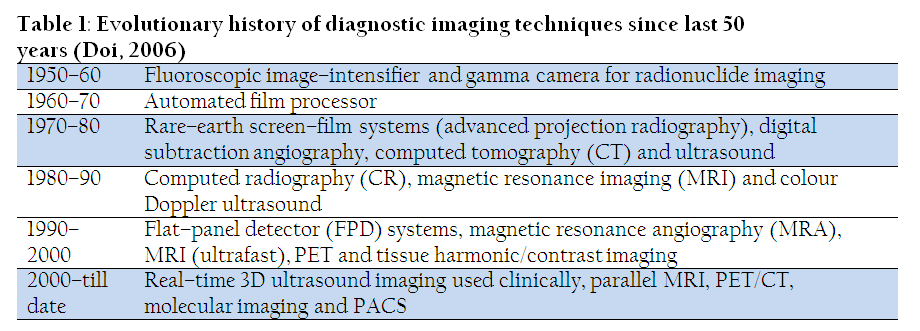
Imaging techniques in medical practice have contributed significantly to the progress of health care since the discovery of x–rays in 1895 (Otto, 1993; Peter, 1995). Medical imaging has gone way beyond the production of images and now has options to display, post–process, record, store, and also of transmission of images, and finally application of picture archiving and communication system (PACS). Thus, image production as earlier was the only option is now only one of many facets of advanced imaging technology (Doi, 2006). This brings together science and technology to create a visual recording of the interior body structures for biomedical research, clinical examination and medical preposition (Olsen et al., 2007). Imaging techniques help to establish a standard database of normal anatomical, physiological and functional parameters that could be used for clinical and research purpose (Thomas and Pickstone, 2007). In the clinical context, medical imaging is generally equated to clinical application of imaging techniques, which includes the x–ray diagnostics, magnetic resonance imaging (MRI), ultrasonography (USG) and endoscopy. X–ray diagnostics normally employ the ionising radiations (x–rays) including projection radiography, fluoroscopy, computed radiography, digital radiography and computed tomography. These x–ray diagnostic techniques differ from each other based on the mode of image acquisition and its storage.
Need for Modern Medical Imaging Systems
Several studies were carried out to determine the sufficiency of screen film images and low quality photo–flouroscopic diagnostic modalities in diagnosis of clinical abnormalities. It was observed that as high as 30% lesions were missed by radiologists and that too mainly by inter–observer variations (Garland, 1949 and 1959; Yerushalmy, 1955). To avoid such problems a need for highly precise and advanced imaging techniques was realised and thus modern diagnostic modalities that possess digitalized system came into existence. However, many other recent studies have reported that clinicians often miss different kinds of lesions even with modern diagnostic modalities like CT (Schmidt et al., 1994; Li et al., 2002, 2005, Armato et al., 2002) and is comparable to the rates reported earlier (Garland 1949, 1959, Yerushalmy 1955), necessitating further advancement in clinical diagnostic imaging techniques. The problem of mis–diagnosis however, can be managed to a greater extent by utilising different imaging techniques that are complementary to each other. Many state of the art diagnostic imaging techniques have been popular in medical field for many years but veterinary practice has seen the development and introduction of new methods for diagnostic imaging only recently (Alkan, 1999; Tan, 2001; Braun, 2003; Kurt and Cihan, 2013).
X–ray diagnostics
Principle
The basic principle for all the x–ray diagnostics is the attenuation of x–rays after encountering any medium. X–rays are produced by bombarding a tungsten target with an electron beam within an x–ray tube (Bushberg et al., 2002). The difference in attenuation along the x–ray beam is responsible for the contrast on the radiographic image. X–rays after passing through the patient get attenuated depending upon the density and thickness of the part to be radiographed. More are the density and thickness of the body parts, greater would be the attenuation. The attenuated x–rays are then acquired and processed for the final image formation. The acquisition and final processing is what differs among the different x–ray diagnostics (Haus, 1996).
Projection Radiography
Radiographic examination of the human body started in 1895 when WC Roentgen produced the first x–ray film image of his wife’s hand (Peter, 1995). Projection radiography utilizes a screen–film system kept into the film cassette that acts as the x–ray detector. X–rays while passing through the patient are being attenuated by interaction with body tissues (absorption and scatter). Attenuated X–rays transmitted through the patient bombard a fluorescent particle–coated screen within the film cassette, thus, causing a photochemical interaction that emits light rays, which expose photographic film within the cassette and produce an image pattern. The film is removed from the cassette and is developed by film processor chemicals. The final product is an x–ray image of the patient’s anatomy on a film (Singh, 1994). The developed film has 2D of several tissues superimposed on each other. Plain radiography has a poor detail of soft tissues, however, several contrast radiographic techniques have been developed to enhance the details of soft tissues during radiography.
Fluoroscopy
Upon projection radiography a particular specific part is being imaged without any information related to the motion. Fluoroscopy in contrast to projection radiography give real–time images of internal body structures by employing a constant input of x–rays but at a lower dose rate compared to that of the conventional radiography. The image of the part that is obtained under fluoroscopy is visible on fluorescent screens. Earlier the main problem with fluoroscopy was a very weak image that could not be stored. However, the development of image intensifier has helped to get better image that can be stored. An image intensifier converts the attenuated radiation into an image. Image intensifier is a large vacuum tube bearing two ends one receiving end (coated with caesium iodide), and the other one a TV camera (Deutschberger, 1955; Rosenbusch et al., 1994). However, the main drawback that limits its utilisation as diagnostic modality is its potential radiation hazard (Shope, 1996).
Digital Radiography
Digital radiography is an x–ray imaging system which differs from the traditional projection radiography in having digital x–ray detectors instead of photographic film (Widmer, 2008). The main advantage associated with the digital detectors is that the PACS can be fully implemented, images can be stored digitally and are available at anytime and anywhere.
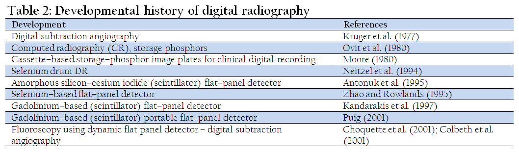
Historical Milestones
Basics of Digital Imaging
There are two types of formats that contain information viz. analog and digital formats. Most of the modern diagnostic imaging techniques like Digital radiography, Nuclear medicine, CT, MRI and Ultrasound acquire information in the form of analog or signal format. However, there are some drawbacks with this format eg. electronic noise that can distort signal and thus there is a need to convert electrical information into digital numbers as computer understands only digital numbers. So it is required to convert the image into digital, which is brought about by an analog to digital convertor (ADC). This conversion of analog signal into digital one is done in the form of binary system under which computers operate. During this conversion, however, some information loss may occur due to quantization and sampling. Quantization loss results due to continuous nature of analog signal while digital image has finite limit, thus digital image represents the rounded–off form of analog signal, though, in medical imaging these information losses are very minute (Jimenez et al., 2008).
The physical principals of digital radiography (DR) do not differ from conventional projection radiography (screen–film radiography). In DR all the conventional X–ray equipments like X–ray machine, table, grid, etc., are same. However, conventional radiography has film which serves both detector as well as storage device while in DR image is generated by digital detectors which is then is stored in digital medium (Widmer, 2008). In general, digital radiography is divided into computed radiography (CR) and direct digital radiography (DDR) (Chotas, 1999; Kotter and Langer, 2002; Mattoon and Smith, 2004; Shepard, 2006). One more digital imaging system i.e., charged coupled devices (CCD) are available which are considered with DDR hardware as image is directly sent to a computer. The main difference that exists between CR and DDR involves image acquisition and not the final result (Widmer, 2008).
Computed Radiography (CR)
CR system bears an image plate (IP), IP reader, an analog to digital converter (ADC), and a computer that process the image (Mattoon and Smith, 2004; Roberts and Graham, 2001; Pizzutiello and Cullinan, 1993). CR begins with the standard x–ray exposure of the patient to acquire the image. is the attenuated x–rays are captured with flexible image plates that contain photosensitive phosphors (containing halogens and activators) (Rowlands, 2002). Commonly used halogen in IP is barium fluorohalide which is doped with activator europium. When an image plate is exposed to X–rays, a latent image is captured together by fluorohalide crystals and activator (Roberts and Graham, 2001). The CR latent image usually dacays very fast as compared with a conventional film–screen system. It may be stable only for minutes to days depending on the type of phosphor used (Rowlands, 2002; Roberts and Graham, 2001; Pizzutiello and Cullinan, 1993). IP reader that processes the latent image consists of laser, optical scanner, photomultiplier tube, and motorized platform which produce visible light (Pizzutiello and Cullinan, 1993). The visible light is then acquired by an optical system coupled to a photomultiplier tube. The tube generates the electrical signals corresponding to the visisble light intensities (Roberts and Graham, 2001; Pizzutiello and Cullinan, 1993). The data in all the above mentioned procedures are in the form of analog system.<>
Direct Digital Radiography (DDR)
DDR readout the image directly barring any intermediate processing step (reader) and thus, possesses an integrated readout property. This leads to a faster image acquisition and thus, beneficial at the places with heavy case load. Direct digital detectors are categorised into flat panel and CCD detectors.
Flat Panel Detectors
Flat panel detectors being rigid in nature have appearance similar to that of film screen system. These detectors are classified as direct (having image plate converting x–ray energy directly into an electrical energy) and indirect (involve two step process for converting x–rays into electrical signals). Finally the digital data that reaches to computer is processed in the same way as described for CR.
Direct Converting Detectors
The direct detector is directly connected to the computer and possesses different layers viz. semi conductor, storage capacitors, thin film transistor arrays (TFT) and a glass substrate (Chotas et al., 1999; Okamura et al., 2002; Dickson, 2003). The thicker topmost photoconductive layer, commonly made up of amorphous selenium, converts X–rays directly to electrical charges. The limited spatial resolution of digital radiography is not due to photoconductive material, amorphous selenium, as it has high intrinsic spatial resolution property but is solely limited by recording and read out devices. Due to the differential charge placed across photoconductor before exposure, electrons that are released migrate perpendicularly to the nearest charge collection electrode connected to the thin film transistors. TFTs are placed beneath the photoconductor and cover entire detector surface in a matrix corresponding to pixels viewed on the computer screen. These TFTs are responsible for read out of charges collected by selenium photoconductor. Storage capacitors are present at higher level, an interface with photoconductive layer and read out electronics are at the lowest level. Read out that occurs row by row is sent to computer after analog to digital conversion (ADC).
There is another type of selenium–based direct conversion DR system known as selenium drum detector. The rotating selenium dotted drum that bears positive surface charge is exposed to X–rays. This exposure leads to development of charge pattern on the drum surface proportional to X–rays which is recorded by analog to digital convertor during rotation. Advantage of these systems is that they provide good quality images compared to those provided by screen–film or CR systems (Neitzel et al., 1994; Bernhardt et al., 1999; Veldkamp et al., 2006; Kroft et al., 2005; Fischbach et al., 2003; Ramli et al., 2005). Also the flat panel detectors can be used for mammography in humans (Zhao et al., 2003).
Indirect Converting Detectors
These detectors convert X–ray energy into electrical charges indirectly. Unlike that of direct converting detectors, it possesses two photoconductive layers viz. a scintillator (made up of structured or unstructured cesium iodide crystals) that is present at the top layer of flat panel below which lay a diode layer (made up of amorphous silicon). The scintillator converts X–rays into visible light which is converted into electric charges by the diode layer. The digitized image is then sent to a computer by the TFT array (pixel), providing true digital output from the detector (Mahesh, 2004).
Charge Coupled Devices (CCD)
Charge coupled technology (Bell Laboratories, 1969) is memory hardware and are popular photodetectors due to their sensitivity to light. CCDs, being the first direct readout detectors used in digital radiography systems, are also used for number of indirect conversion diagnostic imaging applications like fluoroscopy. Due to small size and cost effectiveness, CCDs are popular in digital radiography.
CCD digital imaging system, is a light sensitive sensor for image recording, generally consists of a scintillator, optics for minification, CCD optical detector and in some cases an image intensifier. X–rays after attenuation by the patient interact with the scintillator (such as T1 doped Cesium iodide) and are converted into visible light. Due to the small size of the CCD chip compared to scintillator, an optical coupling is used to minimize the field of light that strikes the CCD chip. CCDs can be used for radiography as part of either a lens–coupled CCD system or a slot–scan CCD system to reduce the field of light. In lens–coupled CCD systems, several CCD chips array form a detector comparable to that of flat–panel detector. In order to fit the projected light on CCD chips optical lenses are used, though, this reduces the number of photons that reach to the CCD and thus leads to higher noise to signal ratio (Chotas et al., 1999). In slot–scan CCD systems (a tungsten anode placed in special x–ray tube), a collimated beam that scan the patient is linked to CCD detector array. The CCD detector chip contains a pixel matrix, polysilicongate and silicon–photosensitive–silicon layers, that develop the electric charges from light photons. Electrical charges in the pixel array are then transformed to digital format.
Conventional Radiography vs Digital Radiography
Digital radiography has numerous advantages over conventional radiography. Some limitations of the conventional radiography include narrow exposure latitude of silver halide systems, need for dark room and processor maintenance, cost of X–ray film and image storage and lack of image post processing capability (Veldkamp et al., 2006). In digital radiography there is convenience of digital image format, no need of X–ray film, processor and chemicals, elimination of filling and storage of X–ray films, improvement in image quality (primarily image contrast), wide latitude for exposures, fewer repeat exposures and rapid image acquisition leading to increased throughput. A significant advantage of digital radiography is that of digital format of the image, which helps in image interpretation at a remote area via internet (teleradiology).
Computed Tomography
Computed tomography (CT) is an imaging technology wherein X–rays are processed by computer to produce tomographic images of scanned area of an object. CT has come a long way since its public inception in 1972 (Kopp et al., 2000). The CT machines have gone through different modifications since its utilization. The machines are generally been up graded in relation to its x–ray source and detector rotations. First generation CT machines had a stationary x–ray tube and the two rotatory detector arrays that would take a scan time of 4.5 min. In second generation CT machines, fan shaped rotating detector array had a 2.5 min scan time possessing multiple detectors. Third generation CT machines had rotating source along with rotation detector array, with a scan time of 18 sec. Fourth generation CT machines possess rotating source with stationary detector array with a scan time of 2 sec. Fifth generation CT machines have stationary source and detector arrays with a scan time of 50 msec (Fox et al., 1998). First generation CT scanners were limited to head scanning only due to long scanning time. The first CT scanner capable of imaging the whole body CT scanner was first was developed by Robert Ledley and installed in 1973 at Minnesota University (Hendee, 1989).
Spiral tomography, an improved tomographic technique, allows continuous rotation wherein an object is slowly and smoothly slid through the X–ray ring to be imaged. Subsequent improvisation of helical CT lead to development of multi–slice CT wherein multiple rows of detectors are used to capture multiple cross–sections simultaneously instead of single detectors (Kalender et al., 1990; Brant–Zawadzki, 2005). In contemporary third or fourth generation scanners only a single slice at a time is acquired (Ambrust, 2007). Currently, another type of CT scanner (Cone beam CT) has been introduced for veterinary diagnostics that possesses image plate rather than detectors thus, cost effective. The image quality and resolution, being at par with the contemporary machines, but it has significantly slower image acquisition rate (Wright, 2014).
Image Formation
Unlike that in digital or projection radiography, X–ray tomographic data is generated using a rotating X–ray source. The X–ray source rotates around the object and the attenuated X–rays are then sensed by the X–ray sensors that are positioned in the opposite direction to that of the X–ray source. Earlier scintillation detectors were used in which photomultiplier tubes were excited by cesium iodide crystals. The cesium iodide was later replaced by ion chambers containing high–pressure Xenon gas in 1980s which in turn were replaced by scintillation systems based on photodiodes instead of photomultipliers. Finally scintillation materials like rare earth garnet or rare earth oxide ceramics with more desirable characteristics are being used (Herman, 2009).
CT being an electronic imaging technique possesses subject image information in the form of current converted from the attenuated x–rays. As the initial x–ray intensity is known, the degree of attenuation by the patient can be inferred by the transmitted intensity at the detectors and thus, by the strength of the resultant signal (Ambrust, 2007). In honour of inventor, the attenuation values are specified in Hounsfield units. The signal generated is sampled, converted into digital form by ADC and is finally processed by the computer and viewed on the screen. Contrast in CT images is due to the variable attenuation of x–rays from different tissues. As with screen film radiography, all the structures that come across the x–ray beam contribute to attenuation during CT imaging. Image display in present day CT scanners need not to be restricted to axial images as they offer isotropic/near isotropic resolution. Instead, images can be piled one upon the other by computer software to produce volume and the images may be displayed in different views (Kalender, 1990; Costello, 1996; Udupa and Herman, 2000).
Artefacts
CT Images give better representation of the object scanned, but susceptibility to a number of artifacts cannot be ruled out and are as follows
Streak Artefact
The streaks are mainly observed in CT images around the hard tissues like bone (posterior brain fossa) and are due to blocking of X–rays by such hard tissues. The streaks may be contributed to number of factors like motion, under sampling, Compton scatter, beam hardening and photon starvation and can be minimized by opting for newer image reconstruction techniques (Boas and Fleischmann, 2011; Jin et al., 2013).
Partial Volume Effect
There is ‘edge blurring’ which develops due to the inability of scanner to differentiate between a low volume of high–density material (e.g., bone) and a larger volume of lower density (e.g., cartilage) (Udupa and Herrman 2000.
Ring Artefact
Ring(s) that appear in an image are perhaps the most common mechanical artefact seen in CT imaging and may be due to detector fault or individual detector element miscalibration (Udupa and Herrman 2000).
Noise
Noise appears as grain over the image and is caused by a high noise to signal ratio. Commonly scanning of a thin slice is the cause but may also develop when an insufficient power is supplied to the X–ray tube, leading to an inadequate energy to the X–rays to penetrate the tissue (Udupa and Herrman 2000).
Motion Artifact
This is generally observed as blurring and is caused by movement of an object being imaged. It might be reduced by using incompressible flow tomographic technique (Nemirovsky et al., 2011).
Beam Hardening
A typical cupped appearance may be seen and occurs due to more attenuation of X–rays that pass through the centre of an object rather than along a path that grazes the edge. This can be corrected by filtration and by computer software software (Van de Casteele et al., 2004; Van Gompel et al., 2011; Jin et al., 2013).
Advantages of CT over Radiography
CT scan has a number of advantages over the conventional radiography. Being tomographic in nature, CT allows sectional or slice oriented imaging of the area scanned, thus eliminating depth perception loss associated with radiography. This helps to get more accurate anatomic localization of the abnormality. Another advantage is that of increased contrast resolution though the spatial resolution is lower. The spatial resolution weakness is however, always overweighed the exceptional contrast resolution in images that are free of superimposed anatomy (Ambrust, 2007).
Magnetic Resonance Imaging
The magnetic resonance imaging (MRI) development can be correlated to the research of Felix Bloch and Edward Purcell who worked independently at Stanford and Harvard Universities, respectively. It was reported that a weak radiofrequency (RF) signal can be emitted by certain nuclei upon application of magnetic field which could yield information about the chemical composition of the material (Hendee, 1989). The credit for the first use of nuclear magnetic resonance as a 2D imaging technique goes to Paul Lauterbur, a chemist at the State University of New York, in 1972 (Lauterbur, 1973; Macovski, 2009). Paul Lauterbur (University of Illinois) and Sir Peter Mansfield (University of Nottingham) were awarded the 2003 Nobel Prize in Physiology or Medicine, reflecting the importance of MRI in Medicine (Moran and Heffernan, 2010).
Magnetic resonance imaging (MRI) as a medical imaging technique is used to investigate the anatomical and physiological function of the body tissues. The technique is widely used in medical hospitals and small animal practice for diagnosis of numerous diseases, staging of the diseases and for follow–up without the risk of exposure to ionizing radiation.
Principle
Unlike other diagnostic imaging techniques, MRI utilises magnetic field produced by MRI scanner to generate images of a particular area or region of a patient’s body. The imaging applications are based on detecting radio frequency signals being emitted by hydrogen atoms in the body that are excited with oscillating magnetic field. This application is as per the Faradays law of induction which states that any change in the magnetic environment of a coil of wire will cause a voltage to be induced in the coil. In other words, a current is induced in the coil if a net magnetic force or flux changes in it (Haacke et al., 1999; Pipe, 1999). During MR scanning, the magnetic field produced by hydrogen atoms is made to pass into and out of the receiver coils and thus, generating a current, which is measured as MR signal. The variation in main magnetic field is used to re–orient of the image for proper visualization. The image contrast is determined by the rate at which excited atoms return to the equilibrium state (McRobbie and Donald, 2007). Image contrast helps to differentiate anatomical structures or pathologies depending upon the potential to attain equilibrium. In every tissue/structure protons return to its equilibrium state or the decay in their induced magnetization after excitation occurs by the independent processes of T1 (spin–lattice) and T2 (spin–spin) relaxation (Johnson et al., 1997; Lauenstein et al., 2004; Brauck et al., 2008).
Spin–lattice relaxation (T1)
T1 weighted image is produced by relaxing of the spin in the transverse magnetization vector after switching off the radio frequency (RF) pulse. To create a T1–weighted image, recovering of different magnetization is first done before measuring any MR signal. This is done by changing the time between each successive RF excitation pulse (repetition time, TR). The image weighting is useful to assess the cerebral cortex, identifying fatty tissue, characterizing focal liver lesions and for post–contrast imaging (Ambrust, 2007).
Spin–spin relaxation time (T2)
T2 relaxation though independent of T1 weighted image occurs in simultaneous to it. T2 relaxation that occurs due to loss in coherence or uniformity of precession rates of spins in the transverse plane is much faster than T1. To create a T2–weighted image, the operator waits for decay in different amounts of magnetization before measuring the MR signal and is done by changing the echo time (TE). The image weighting is useful for detecting edema, revealing white matter lesions and assessing zonal anatomy in the prostate and uterus (Ambrust, 2007).
APPLICATION
Magnetic Resonance Angiography (MRA)
As the name suggests MRA is useful in evaluating the arteries in health or in diseased conditions. Various techniques are being utilised to generate arterial images like administration of a paramagnetic contrast agent (gadolinium) or a flow–related enhancement (e.g., 2D and 3D time–of–flight sequences). In both the above techniques, the image signal is mainly due to recently passed blood. Other techniques, that involve phase accumulation also known as phase contrast angiography, can also be used to generate flow velocity maps easily and accurately. Magnetic resonance venography (MRV) like MRA is used to image veins wherein the tissue is excited inferiorly and the signal is gathered in the plane immediately superior to the excitation plane (Haacke et al., 1999).
Functional MRI (fMRI)
fMRI gives the pattern of changing neuronal activity in the brain. The brain is scanned at lower spatial resolution but at a higher temporal resolution (every 2–3 seconds) when compared to anatomical T1 weighted imaging. Increases in neural activity cause changes in the MR signal via T*2 changes (Thulborn et al., 1982), generally termed as BOLD (blood–oxygen–level dependent) effect. Increased neural activity as require more oxygen and is met by vascular system leading to the increased amount of oxygenated hemoglobin relative to deoxygenated hemoglobin. As the deoxygenated hemoglobin attenuates the MR signal, the vascular response thus, leads to a signal increase and is related to the activity of neurons. The BOLD effect also allows the generation of high resolution 3D maps of the venous vasculature within neural tissue.
Interventional MRI
Owing to lack of any harmful effect MRI is well–suited for interventional imaging, wherein the images are used to guide minimally invasive procedures though without using any ferromagnetic instrument. Interventional MRI is being developed as a specialised discipline in which the MRI is used in intra–operative surgical procedures (Leblanc et al., 1999). Currently specialized MRI systems are also now available that allow imaging simultaneously with the surgical procedure. However, the surgical procedure is temporarily interrupted in order to verify images for the success of the procedure (Lipson et al., 2001).
Clinical Interpretations
The tissue contrast in MRI may vary due to multifactorial causes and a standardized grey scale is not possible (Wherli and McGowan, 1996).
No Signal Tissue
Substances having minimal or no hydrogen atom appear signal void such as gas, dense cortical bone, calcified areas, implanted materials or rapidly flowing blood (Lufkin, 1998). Arterial blood vessels also appear signal void on spin echo images due to faster speed of blood (Ambrust, 2007).
Structures with Different T1 and T2 Intensities
Fluid when compared to solid but Juicy water based tissues (inflammatory, edematous, necrotic and most tumours) have different intensities for T1 and T2 weighted images (Tidwell, 2007). Most solid but juicy water based tissues have long relaxation times (Elster and Burdette, 2001). These lesions appear hyperintense against a background of darker normal tissues on T2 weighted image. This is the reason that the T2 weighted images are known as pathology scans (McRobbie et al., 2003). However, fat stores that appear bright on T1 weighted images may not appear dark on T2 weighted images. This is due to its short T1 relaxation rate and an intermediate T2 relaxation rates (Lufkin, 1998; Hashemi and Bradley, 1997; Elster and Burdette, 2001).
SAFETY CONCERNS OF MRI
Implants
Patient reviewing is must for MRI and the implants that a patient might carry are grouped as MR–Safe implants, MR–conditioned implants and MR–unsafe implants. MR–safe implants include non–magnetic, non–electrically conductive, and non–RF reactive implants, which do not pose any threat during an MRI procedure.
MR–Conditional implants include magnetic, electrically conductive that are safe for operations (conditions defined) in proximity to the MRI, such as 1.5 tesla field safe implants.
MR–Unsafe implants include ferromagnetic items that directly pose danger to the persons and equipment within the magnet room (ASTM, 2005)
Genotoxic Effects
So far no biological harm from even very powerful static magnetic fields has been proven (Formica and Silvestri, 2004; Hartwig et al., 2009). However, some genotoxic effects of MRI scanning have been demonstrated under in vivo as well as in vitro conditions (Suzuki et al., 2001; Simi et al., 2008; Lee et al., 2011; Fiechter et al. 2013). A recent review on safety of MRI has recommended a need for further studies as a precautionary principle (Hartwig et al., 2009). One genotoxic study had reported that MRI in comparison to techniques utilising the ionising radiations lead to comparable DNA damage. Thus, the DNA damage mechanisms though may be different but cannot be ruled out with MRI and need be elucidated (Knuuti et al., 2013)
Peripheral Nerve Stimulation (PNS)
Rapid on and off switching of magnetic field gradients is supposed to cause nerve stimulation exhibited in twitching sensation especially in the extremities (Cohen et al., 1990; Budinger et al., 1991).. The peripheral nerves are possibly stimulated by magnetic field due to the gradient coils (Reilly, 1989)..Although PNS had not been a problem for the slow, weak gradients used in the early days of MRI, the strong, rapidly switching gradients used in techniques such as EPI, fMRI, diffusion MRI, etc. can induce PNS.
Pregnancy
Although adverse effects of MRI on the foetus have not been demonstrated (Alorainy et al., 2006) but present guidelines does not recommended pregnant animal/woman to undergo MRI unless essential. This is particularly important during the organogenesis that is during the first trimester of pregnancy. During MRI scanning foetus may be more sensitive to heating and noise effects apart from other general concerns. The use of contrast medium (gadolinium based) is an off–label indication in pregnancy. It may only be used in the lowest required dose that is sufficient to provide useful diagnostic information (Webb and Thomsen, 2013).
Claustrophobia
MRI scans can be problem for claustrophobic human patients though not in animals as scanning is done under general anaesthesia. In human beings however, availability of open or upright systems, though produce inferior scan quality, have now avoided such complicacy.
CT Scan vs MRI
CT scan is an ionising x–ray technology that relies upon the attenuation of x–rays by the tissue to be scanned while MRI is a non–ionising technology that relies upon magnetic field and radiofrequency for hydrogen mapping of the tissue. Image acquisition in CT scan occurs in transverse plane having a minimal slice thickness of 0.5mm while in MRI image can be acquired in any plane with slightly thicker slice (2.0mm). The scanning time is lower (seconds to minutes) in CT while scanning in MRI is usually slower (30–60minutes). The contrast material used is iodinated contrast media in CT and Gadolinium based paramagnetic contrast media in MRI. MRI provides great imaging details of soft tissue and CT of osseous tissue (Labruyère and Schwarz, 2013). MRI of head for disorders like neoplasms, vascular disease, intracranial pressures, cervicomedullary lesions, etc. is superior in comparison to CT scans (Brenner and Hall, 2007; Semelka et al., 2007; Evans, 2009). Exposure to ionizing radiation risk associated with CT scan is not a problem with MRI (Evans, 2009). CT scans in absence of MRI may be utilised to diagnose headache or in emergency settings when hemorrhage, stroke or traumatic brain injury are suspected (Semelka et al., 2007; Evans, 2009). CT scan of the head should preferably be avoided in emergency situations, when a head injury is minor (Haydel et al., 2000; Marion, 2005; Stiell, 2005; Andy et al., 2008).
Nuclear Medicine Imaging
Nuclear medicine scintigraphy is a diagnostic technique that requires gamma emission radioisotope (radiopharmaceutical agent). Henri Becquerel radioactivity discovery two months later too was a serendipitous (Graham et al., 1989). But it was Georg de Hevesy who applied the radioisotopes to the study of plant and animal metabolism (Hevesy, 1923), which later earned him Nobel Prize in 1943 (Moran and Heffernan, 2010). When compared to radiography, development of imaging nuclear medicine took some time and the main reason was unavailability of radioactivity detectors. In 1928 Geiger–Mueller tube were introduced that were capable to detect radioactivity though relatively insensitive (with an efficiency of appox. 2%) and still required a high dose of activity to be injected (Blahd, 1979; Edwards, 1979). In 1935, radioisotope (P–32) distribution in the animal body (rat) was first studied by de Hevesy and Chiewitz (Hevesy, 1939). The development of gamma camera by Anger leads to the significant development of scintigraphic imaging (Anger, 1958).
A standard gamma radiation–emitting isotope should have a short physical half–life, a chemical structure suitable for better labelling of different tissues/organs, and economical as well. The most frequently used isotope, 99mTechnetium (99mTc), bears almost all the above mentioned characteristics (Balogh et al., 1999). Radiopharmaceutical agents are formulated in various physicochemical forms (radioisotope with the base material), to deliver the active atoms to the particular organ of tissue. Once localized in the tissue of interest, the gamma radiation is emitted from the radiopharmaceutical, which is detected and measured externally. The main difference between nuclear scintigraphy and other radiologic tests is that former gives functional assessment of organs whereas the latter methods give anatomical description. The advantage of assessing the function of an organ is that it helps physicians in making a diagnosis regarding the functional capacity of the particular organ.
Principle
The principle of nuclear medicine scintigraphy is based on detection of radiations by the gamma camera. Gamma photon upon interaction with a thallium doped sodium iodide detector material loses energy in the form of excitation. The incident gamma photon can be partially (Compton Effect) or totally (photoelectric effect) absorbed with latter being the actual phenomenon typical to the gamma–ray emission site. The photons generated are collected by the photocathode of a photomultiplier tube (Anger, 1958). The secondary light photons generated in the crystal after interaction with the incident gamma radiations are detected by a photomultiplier tube (PMT) and are converted to electrons. The electrons are accelerated and multiplied by ten dynodes and finally collected by an anode where electrical impulse, proportional to energy level of photons, is generated. The output signal amplitude after amplification by the PMT is measured, digitized and finally stored. Unlike the light, the gamma rays cannot be focussed by lenses and a special kind of collimator is used to direct them towards the crystal (Anger, 1964). The final scintigraphic image corresponds to the distribution of radioactivity on the crystal detector and gives the physiological activity of the tissue.
Now–a–days, advanced nuclear imaging techniques like whole body and single photon emission computer tomography (SPECT) use SPECT–camera. In SPECT the computer moves the detector to give better picture resolution, sensitivity and 3D radiopharmaceutical distribution.
Indications for Scintigraphy
Skeletal scintigraphy is the most commonly per¬formed scintigraphy (or bone scanning) procedure in veterinary practice. It offers high sensitivity for detecting early disease, and the ease of evaluation of the entire skeleton (or a region) makes it an ideal tool for screening cases of obscure or occult lameness. However, Scintigraphy can be used to look at a variety of organ functions including brain, heart, lung, kidney, liver, thyroid etc (George and Taylor, 2004; Hindie et al., 2007; Scarsbrook et al., 2007).
Limitations
The major limitation with nuclear imaging is of the large dosage of radionuclide (Moran and Heffernan, 2010). Apart from dose to the patient, it may not detect the early stages of metastatic disease and myeloma (Schimdt et al., 2009). Low spatial resolution and commonly encountered false positives due to degenerative disease or trauma are other few limitations. Thus, whole–body imaging in nuclear medicine often remains confined to specific organ imaging or of tumors (Moran and Heffernan, 2010).
Diagnostic Ultrasound
Ultrasound is high frequency sound wave (>20 KHz) that is used to produce the image of the body. For diagnostic purposes, frequency range usually ranges from 2 to 10 MHz, though higher frequencies are used in advanced techniques. Sound waves are longitudinal waves wherein the direction of travel of particles within the wave occurs similar to that of the wave. As the sound wave is mechanical energy, it requires the medium to propagate unlike that of the light and radio waves.
Ultrasound transmits energy by alternating regions of rarefaction (low pressure) and compression (high pressure) (Powis, 1986; Bushberg et al., 2002). Each wave has an associated speed of travel (velocity), wavelength and frequency. Velocity is the rate at which sound travels through an acoustic medium and is determined by physical density and hardness of the transmitting medium (Bushberg et al., 2002). Velocity increases as stiffness increases provided the physical density remains constant. As a general rule the velocity of sound waves through solids, liquids and gases is highest, lower and lowest, respectively. Wavelength is the distance travelled by a sound wave in one cycle and is measured in millimetres in diagnostic ultrasound. Its importance lies in the image resolution and higher the wavelength lesser will be image resolution. Frequency is the number of cycles (combination of compression and successive rarefaction) a wave travels per second. The relationship of above mentioned three factors is as under
Velocity (V) |
= Frequency (F) |
× Wave length (λ) |
In general the speed of sound through soft tissues is taken as constant value (appx. 1540 m/s), so the wavelength and frequency are inversely related to each other.
Ultrasound wave Interaction with the Tissues
The ultrasound beam produced in the form of pulse from the piezoelectric crystal is returned back to the tissues in the form of an echo. This phenomenon of sound wave production in the form of a pulse and its echo returning back is referred to as pulse echo principle. As the sound wave interacts with the tissue interface, the sound wave may be reflected, refracted or scattered depending upon the differences in acoustic impedance of the tissues. Acoustic impedance is the resistance to the flow of sound through a medium, affected by the density and stiffness of the medium and is independent of the frequency as given below
Acoustic impedance (Z) = Tissue density (D) × Velocity (V)
The amplitude of returning echo corresponds to the difference in acoustic impedance. If large difference exists between different tissues, larger reflection of the sound waves occurs and lesser waves get transmitted. Conversely, if no difference in acoustic impedance exists between the tissues no echo is formed.
Among the most commonly encountered medium/tissue, gas and bone has largest difference in acoustic impedance. These interfaces reflect almost all the sound waves and little of negligible amount of sound waves pass through them. Though the speed of sound increases as the density of the medium increases but due to inability to compress or rarefy the sound wave in bone, impedance to sound transmission is high. This total reflection of sound waves at these interfaces creates a shadow below and thus, speed of sound in bone or gas filled lung is not clinically important. In order to do better scanning, it is therefore essential to apply a coupling gel between the tissue and transducer to prevent trapping of air.
When a patient is scanned it is must to keep the transducer perpendicular to the tissue as the angle of incidence of sound waves should be 90 degrees to the reflector surface. Angle of incidence is the angle at which sound waves encounters the medium/tissue. When a sound wave is kept perpendicular to the tissue surface, the reflected sound wave returns back in a reverse direction (180 degrees) and reaches the transducer. If the angle of incidence is not perpendicular, angle of reflection equals the angle of incidence and if the sound wave strikes the reflecting surface farther than 3 degrees, it is quite likely that the echo will not reach to the transducer.
When a sound wave travels through the medium, it gets attenuated, which is determined by the distance travelled and frequency of the sound wave. Attenuation is higher in high frequency wave and increases as the distance travelled is increased. Attenuation involves three components viz. reflection, absorption and scattering. The reflection occurs when the sound wave encounters the tissues of different acoustic impedance and is responsible for producing the image after returning back to the transducer. This reflection would decide the intensity of the image. Greater is the amount of reflected sound waves reaching the transducer, brighter would be the image. Absorption, the main component of attenuation in soft tissues occurs due to conversion of sound wave’s mechanical energy into heat energy, though it is relatively low with diagnostic ultrasound amount. Scattering occurs as the sound wave encounters small, irregular surfaces. It increases with the increase in frequency of the sound wave. Scattering occurs mainly within the parenchyma of organs and is responsible for their texture in the image (Bushberg et al., 2002).
Ultrasound Generation and Detection
In diagnostic ultrasound, piezoelectric crystals present in transducer are used to convert electrical energy into sound waves and then upon echo sound waves are converted back to electrical energy (Kremkau, 1998). A typical transducer emits sound waves for less than 1 % of the scanning time and receives the same for more than 90 % of the scanning time (Herring and Bjornton, 1985; Nyland et al., 2002), but cannot send and receive sound waves at the same time (Curry et al., 1990). Transducers are available in different shapes. Selection of a transducer for scanning depends upon its physical properties and anatomic structure to be imaged. There are mainly two types of transducers available, mechanical and electronic, depending upon the presence or absence of moving parts. In mechanical transducers actual movement of a single or multiple crystals determines the coverage of the volume of the tissue (Nyland et al., 2002). The crystals, immersed in acoustic coupling medium, move back and forth or rotate within the transducer head. These type of transducers produce sector images. Electronic transducers (array transducers) are composed of several small elements with various arrangements. Transducer elements may be arranged in curved line (Convex array), line or rectangle (linear array) or concentric rings (annular array) (Kremkau, 1998). Electronic transducers do not possess moving parts and also do not need coupling gel, and the images of different shapes are produced by electronically firing the elements in various sequences. It is the most commonly used transducer in ultrasound machines.
Two main basic shapes of ultrasound images include sector and rectangular. Sector images are often produced by transducers having small contact area (small footprint) and rectangular images are produced by transducers with large footprint. For thoracic imaging sector transducers are beneficial than linear ones as the image is acquired through a small contact area of intercostal spaces. For abdominal or other soft tissue structures transducer selection depends upon sonologist’s preference.
Image Display
There are three modes of echo display viz. A mode, B mode and M mode. B and M modes are most commonly used for ultrasonography (Gugjoo et al., 2014). A mode imaging is generally restricted for eye imaging. The most commonly used format for imaging is B mode while M mode is most commonly used for echocardiography. B mode images are collection of dots corresponding to strength of the returning echoes. (Herring and Bjornton, 1985; Rantanen and Ewing, 1981). Dots are being displayed on black background, with brightest dot corresponding to stronger returning echoes. Depth of the structure that is returning echoes is represented by the depth of dots relative to the transducer. M–mode is most commonly used in echocardiography to quantitatively evaluate the function of cardiac chambers as well as valves. M–mode imaging region is selected by a cursor on the B mode image with depth of the image being displayed on vertical axis and time on horizontal axis.
Image Interpretation
Image on the screen is read by its echogenicity with brighter structure represented by hyperechoic and darker structure as anechoic. Structures with same echogenicity are isoechoic. Liquids generally appear black (anechoic) and bone or air as bright (hyperechoic). Soft tissue has different degrees of echogenicity.
Artefacts
Although in ultrasonography, artefact may sometime enhance the evaluation, as in fluid–filled structures but normally should be prevented. Few of the common artefacts of sonography are listed below (Tod Drost, 2007).
Mirror Images
These artefacts are produced by highly reflective surfaces and are commonly encountered when liver is imaged against the highly reflective surfaces like diaphragm/lung (Tod Drost, 2007).
Reverberation
These are multiple hyperechoic foci that occur at regular intervals on the image. These are encountered at highly reflective surfaces when there is bouncing back and forth of the sound waves between transducer and reflective surface. Commonly it is seen in abdominal sonography of intestinal gas.
Acoustic Shadowing and Acoustic Enhancement
These are regions of increased and decreased echogenicity distal to high reflective and low attenuation areas, respectively. Physical acoustic shadowing is common at soft tissue/bone or soft tissue/air interfaces while pathological shadowing is seen with calculi (renal, cystic or cholecystic). Acoustic enhancement is seen distal to fluid filled structures (gall/urinary bladder).
Side Lobe and Grafting Lobe
Side lobe and grafting lobe artefacts are secondary sound beams that arise in different direction than the primary sound beams. These artefacts can arise from all the available transducers while grafting lobe can arise from array transducers. Both these lobes result in an error in positioning of the returning echo. As these lobes are weaker than the primary sound beams, they must encounter the highly reflective surface in order to be noticed.
Doppler Sonography
Doppler sonography applies the principle of Doppler shift, which implies an apparent change in the pitch or sound wave frequency with the change in the positioning of the reflector. This effect is named after an Austrian mathematician and Physicist, Johann Christian Andreas Doppler, who proposed this effect in 1842. In sonography, most common reflector is red blood cells (Bushberg et al., 2002). The Doppler shift is difference in frequency between the incident sound waves and reflected waves (Gugjoo et al., 2014). Doppler frequency shift being recorded in Hertz is in audible range compared to sonographic frequency recorded in Megahertz. Maximum Doppler effect is obtained when sound beam is parallel to the moving reflector. However, practically sound waves are rarely parallel to the blood flow direction. So in order to correct the effect of angulation, Doppler angle is used in various calculations (Nyland et al., 2002).
Doppler Modes
There are four Doppler modes viz. continuous–wave Doppler, pulsed–wave Doppler, colour Doppler and power Doppler. In continuous wave Doppler two separate crystals are used wherein one continuously emits sound waves and other continuously receives echoes (Bushberg et al., 2002). Due to continuous sampling much higher velocities can be recorded with continuous wave Doppler, which makes it highly accurate for measuring Doppler shift. The main problem with continuous wave Doppler is that it measures all Doppler shifts that comes along the path of the sound wave and thus, differentiation of blood flow velocity from different vessels is not possible. In pulsed wave Doppler, same crystal is used to send as well as to receive the sound waves (Bushberg et al., 2002). Generally pulsed wave Doppler is used in combination with B mode, known as Duplex Doppler (Bushberg et al., 2002; Nyland et al., 2002; Gugjoo et al., 2014). With B–mode, a particular vessel is selected for Doppler interrogation and an electronic gate (region of frequency sampling) is positioned over the blood vessel. This gate helps in receiving echoes from particular region on the basis of time taken for sound waves to reach the structure and for echoes to return back to the transducer. Due to the feature of selection of particular vessel, it can be used to evaluate blood velocity in a single vessel. Both the continuous and pulsed wave Doppler produce spectral tracing, that records velocity and direction of blood flow as a function of time. Spectral tracing can be broad or thin depending upon the character of flow velocity. If there is large range of blood flow velocity within the sample area, spectral tracing would be broad while if homogenous blood flow velocity is present, spectral tracing would be thin. Colour Doppler, a variation of pulsed wave Doppler (Bushberg et al., 2002; Nyland et al., 2002; Gugjoo et al., 2014), records blood flow velocity at multiple areas within an image and then the velocities are colour coded. Red and blue colour is commonly used for colour Doppler with former representing the blood flow towards the transducer while latter represents the flow away from transducer, though it may vary. Colour Doppler is angle dependant and at 90 degrees the Doppler shift recorded is zero. The main limitation with colour Doppler is that mean velocity is displayed and only limited maximum velocity can be displayed (Nyland et al., 2002). Power Doppler analyzes total strength of Doppler signal but without direction (Bushberg et al., 2002). It creates a colour map of the Doppler shift where hugeness and brightness represent the power of the Doppler signal. The main benefit of power Doppler compared to colour Doppler is that it can detect very low velocity blood flow, is independent of Doppler angle and is not prone to aliasing artefact (Rubin et al., 1994).
Artefacts of Doppler sonography
In pulsed wave Doppler, aliasing results when pulse repetition frequency (PRF) is very low and on spectral tracing a portion of the tracing appears on the opposite direction and thus displayed on wrong side of base line (Bushberg et al., 2002; Nylan et al., 2002). In colour Doppler, it is seen as addition of colour from opposite side of the colour scale. To correct the aliasing, PRF should be increased and sampling rate needs to be twice the highest frequency as the returning blood flow (Nyland et al., 2002). The other way to decrease the aliasing in spectral tracing is by changing the base line. Range ambiguity occurs when PRF is too high such that all the returning echoes are not received before the next pulse is sent (Nyland et al., 2002). This results in interpretation of lagging echoes being closer to transducer than they actually are. This leads to production of Ghost images, though generally not interfering with image interpretation.
3D and 4D Ultrasound
3D and 4D ultrasounds are medical ultrasound techniques that provide three–dimensional images of the part to be scanned. The main difference in 3D and 4D ultrasound is of time; former providing delayed images while the latter provides real time images. 3D ultrasound was first developed by Olaf Von Ramm and Stephen Smith at Duke University in 1987 (Von Ramm and Smith, 1984).
Principle
Unlike that of the 2D ultrasound in which the sound waves are sent and received in straight direction, the sound waves in 3D/4D are sent at different angles. The returning echoes are processed by computer program in such a way to give three–dimensional image volume especially of the fetus, and are comparable to CT scan machine image construct. Clinical use of this technology is an area of intense research activity especially in fetal anomaly scanning (Benacerraf et al., 2005; Benoit and Chaoui, 2004; Krakow et al., 2003) but there are also popular uses that have been shown to improve fetal–maternal bonding (Ji et al., 1997)
Tissue Harmonic Imaging
Tissue harmonic imaging (THI) is a new grey scale sonographic imaging technique that can provide superior quality image compared to conventional sonography (Tranquart et al., 1999). Images are derived from the higher frequency, especially second harmonic sound, as the ultrasound pulse passes through the body tissue (Muir and Carstensen, 1980; Staritt et al., 1985, 1986). In THI, the conventional echoes generated from the tissues are eliminated and only harmonic frequencies are used to form the image (Tranquart et al., 1999). On theoretical basis, THI offers number of benefits over pulse–echo imaging viz. increased penetration without the loss in detail, improved contrast resolution, reduced noise and clutter, better lateral resolution, thinner slices, and reduced artefacts (side lobes, reverberations) (Shapiro et al., 1998; Tranquart et al., 1999).
Ultrasonography vs Radiology
Ultrasonography in contrast to conventional x–rays examinations distinguishes well between soft tissues and is preferred for soft tissue examinations like abdomen including the obstetrical applications. In relation to skeletal tissue (bone) and pulmonary tissue, ultrasonography is least preferred as the sound waves cannot pass through the air/gas and the bony tissue. This also restricts the application of ultrasound in the brain examination except in young ones where fontanels are still open.
Endoscopy
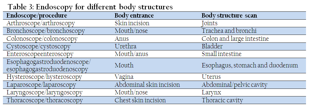
The word endoscopy is derived from the Greek word endoscopesis, which means to watch inside carefully (Antoniou et al. 2012). Thus endoscopy is a type of input device with a miniature wireless video camera that sends images to monitor inside structures of the body without any surgery. Though endoscopic examinations had been performed since the 5th century BC, the term endoscopy was first encountered in medical manuscripts in 19th century AC, following the evolution of novel instruments and artificial light (Antoniou et al. 2012). Earlier in its development, the technique was limited by its capability to reach deep inside due to absence of flexible endoscope. Later in 1960s, discovery of fiber optics revolutionized the capability of endoscopy to visualize almost all the structures deep inside the body with relatively small and painless devices (Nordqvist, 2009). Currently, many different kinds of endoscopes have been developed that help to image almost all the internal body structures. Most commonly used are are lighter with a small video camera on the end that puts pictures on a computer screen. Endoscopes may be stiff or flexible and can vary in length and shape. Now–a–days endoscopy is one of the important diagnostic and surgical tools being used in zoological medicine (Burrows and Heard, 1999).
Endoscopy is performed by inserting the endoscope in the particular area unlike the imaging tests, like x–rays and CT scans which used radiations for imaging. Endoscopes can get pictures of the body parts they can reach. But some types of endoscopy can also be used to help get better, more detailed information employing ultrasounds (Lecoindre and Chevallier, 1997) and are used to find the stage (extent) of cancer. Endoscope may be put in the mouth, anus, or urethra or may be put through small incision made in the skin.
Components of an Endoscope
An endoscope normally comprises a rigid or flexible tube, a light source, generally outside the body, to illuminate the organ under inspection. Generally the image from the objective lens to the eye piece is transmitted via optical fibre system. It may be a relay lens system (rigid endoscopes) or a bundle of fiberoptics (fiberscope). Modern instruments now have the additional channels for insertion of medical instruments and options for video storage of the procedures.
The main limitation associated with endoscopy is need of anaesthetising the animal. It’s also limited in its application in assessing the motility of the organ (Simpson, 1993).
Availability of Imaging Techniques in Veterinary Practice
Over the last 2 decades, use of advanced imaging modalities, such as CT and MRI, has become more frequent in veterinary medicine especially in developed countries. However, the developing countries, like India, still have dearth of such advanced techniques in veterinary practice. In regular veterinary practice, survey radiographs and ultrasound are primary imaging modalities being easily available, cost effective and without any need for general anaesthesia which may be a limitation in advanced imaging. However, CT and MRI play an essential role especially in cases where anaesthesia has no deleterious effect and cost is not a factor. The main reason for limited availability of advanced imaging in veterinary practice include the heavy initial expenses which are difficult to recover in general veterinary practice, maintenance costs, lack of expertise for interpretation, requirement of specialized training and technical staff and need of adjustable machines to accommodate the range of animal sizes (Ibrahim et al., 2012; Wright, 2014). There are several reports on the application of human CT and MRI set ups for diagnostic imaging in animals. As the awareness among the animal owners is increasing there would be more demand of such advanced diagnostic imaging modalities in veterinary practice. It is expected that some of the advanced diagnostic imaging facilities would be available at least at veterinary teaching and research Institutes in near future.
REFERENCES
Alkan Z (1999). Veterinary Radiology, 1st ed., Mina Ajans. Ankara, 121–146.
Alorainy IA, Albadr FB, Abujamea AH (2006). Attitude towards MRI safety during pregnancy. Ann. Saudi Med. 26 (4): 306–309.
PMid:16885635
Ambrust LJ (2007). Digital images and digital radiographic image capture. In: Textbook of Veterinary diagnostic radiology, Thrall, DE. Saunders, Elsevier. 22–37.
Andy JS, Jeffrey BJ, John BJ, Stephen CV, Alisa GD, Patricia HK, Jamshid G, Silvana R, David WW, Robert WL, Aric B, Paula B, Marlena WM, Rhonda WR (2008). Clinical Policy: Neuroimaging and Decisionmaking in Adult Mild Traumatic Brain Injury in the Acute Setting. Ann. Emerg. Med. 52(6): 714–748.
http://dx.doi.org/10.1016/j.annemergmed.2008.08.021
PMid:19027497
Anger HO (1958). Scintillation Camera. The Review of Scientific Instruments. 29(1): 27–33.
http://dx.doi.org/10.1063/1.1715998
Anger HO (1964). Scintillation camera with multichannel collimators. J. Nucl. Med. 5: 515–531.
PMid:14216630
Antoniou SA, Antoniou GA, Koutras C, Antoniou AI.(2012).Endoscopy and laparoscopy: a historical aspect of medical terminology. Surg. Endosc. 26(12):3650–4.
http://dx.doi.org/10.1097/SLE.0b013e3182747ac2
PMid:23238375
Antonuk LE, Yorkston J, Huang W, et al (1995). A realtime, flat–panel, amorphous silicon, digital x–ray imager. Radio Graph. 15: 993–1000.
Armato SG III, Li F, Giger ML, MacMahon H, Sone S, Doi K (2002). Performance of automated CT nodule detection on missed cancers from a lung cancer screening program Radiol. 225: 685–692.
ASTM International (2005). American Society for Testing and Materials (ASTM) International, Designation: F2503–05. Standard practice for marking medical devices and other items for safety in the magnetic resonance environment.
Balogh L, Andócs G, Thuróczy J, Németh T, Láng J, Bodo K, Janoki GA. (1999). Veterinary Nuclear Medicine. Scintigraphical examinations – a review. Acta Vet. Brno. 68: 231–239.
http://dx.doi.org/10.2754/avb199968040231
Benacerraf BR, Benson CB, Abuhamad AZ, Copel JA, Abramowicz JS, Devore GR, Doubilet PM, Lee W, Lev–Toaff AS, Merz E, Nelson TR, O'Neill MJ, Parsons AK, Platt LD, Pretorius DH, Timor–Tritsch IE (2005). Three– and 4–dimensional ultrasound in obstetrics and gynecology. J. ultrasound Med. 24(12): 1587–1597.
http://dx.doi.org/10.1002/uog.2016
http://dx.doi.org/10.1002/uog.2134
Benoit B, Chaoui R (2004). Three–dimensional ultrasound with maximal mode rendering: a novel technique for the diagnosis of bilateral or unilateral absence or hypoplasia of nasal bones in second–trimester screening for Down syndrome". Ultrasound Obstetr. Gynecol. 25(1): 19–24.
http://dx.doi.org/10.1002/uog.1805
PMid:15690554
Bernhardt TM, Otto D, Reichel G, Ludwig K, Seifert S, Kropf S, Rapp–Bernhardt U (1999). Detection of simulated interstitial lung disease and catheters with selenium, storage phosphor, and film based radiography. Radiol. 213: 445–454.
http://dx.doi.org/10.1148/radiology.213.2.r99nv20445
PMid:10551225
Blahd WH (1979). History of external counting procedures. Semin. Nucl. Med. 9(3): 159–163.
http://dx.doi.org/10.1016/S0001-2998(79)80025-2
Boas FE, Fleischmann D (2011). Evaluation of Two Iterative Techniques for Reducing Metal Artifacts in Computed Tomography. Radiol. 259(3): 894–902.
http://dx.doi.org/10.1148/radiol.11101782
PMid:21357521
Brant–Zawadzki MN (2005). The role of computed tomography in screening for cancer. Eur. Radiol. 15(suppl 4): D52–D54.
http://dx.doi.org/10.1007/s10406-005-0115-8
PMid:16479647
Brauck K, Zenge MO, Vogt FM, Quick HH, Stock F, Trarbach T, Ladd ME, Barkhausen J (2008). Feasibility of whole body MR with T2– and T1–weighted real–time steady–state free precession sequences during continuous table movement to depict metastases. Radiol. 246(3): 910–916
http://dx.doi.org/10.1148/radiol.2463062017
PMid:18187400
Braun U (2003). Ultrasonography in gastrointestinal disease in cattle. Vet. J. 166: 112–124.
http://dx.doi.org/10.1016/S1090-0233(02)00301-5
Brenner DJ, Hall EJ (2007). Computed Tomography – an Increasing Source of Radiation Exposure. New England J. Med. 357(22): 2277–2284.
http://dx.doi.org/10.1056/NEJMra072149
PMid:18046031
Budinger TF, Fischer H, Hentschel D, Reinfelder HE , Schmitt F (1991). "Physiological effects of fast oscillating magnetic field gradients". J Comput Assist Tomogr 15(6): 909–914.
http://dx.doi.org/10.1097/00004728-199111000-00001
PMid:1939767
Burrows CF, Heard DJ (1999). Endoscopy in non–domestic species. In: small animal endoscopy, Tams TR (eds). Mosby, St Louis, MO, 297–421.
Bushberg JT, Anthony SJ, Edwin LM, John BM (2002). The essential physics of medical imaging. Lippincott Williams & Wilkins. 38.
Bushberg JT, Seibert JA, Leidholdt EM, Boone JM (2002). The essential physics of medical imaging. 2nd ed., Philadelphia, Lippincott Williams and Wilkins, 469–554.
Choquette M, Demers Y, Shukri Z, Tousignant O. Aoki K, Honda M, Takahashi A, Tsukamoto A (2001). Performance of a real–time selenium–based x–ray detector for fluoroscopy. Proc SPIE. 4320: 501–508.
http://dx.doi.org/10.1117/12.430873
Chotas HG, Dobbins JT, Ravin CE (1999). Principles of digital radiography with large–area, electronically readable detectors: a review of the basics. Radiol. 210: 595–599.
http://dx.doi.org/10.1148/radiology.210.3.r99mr15595
PMid:10207454
Cohen MS, Weisskoff RM, Rzedzian RR, Kantor HL (1990). Sensory stimulation by time–varying magnetic fields. Magn. Reson. Med. 14(2): 409–414.
http://dx.doi.org/10.1002/mrm.1910140226
PMid:2345521
Colbeth RE, Boyce SJ, Fong R, Gray KW, Harris RA, Job ID, Mollov IP, Nepo B, Pavkovich JM, Taie–Nobarie N, Seppi EJ, Shapiro EG, Wright MD, Webb C, Yu JM (2001). 40 x 30 cm flat–panel imager for angiography, R&F, and cone–beam CT applications. In: Medical Imaging. Physics of medical imaging. San Diego. CA. 94–102
Costello P (1996). Subsecond scanning makes CT even faster. Diagn.Imaging 18:76–79.
Curry TS III, Dowdy JE, Murry RC Jr (1990). Ultrasound. In: Christenson's physics of diagnostic radiology, Ed. Curry TS III, Dowdy, JE, Murry RC Jr, 4th ed., Philadelphia, Lea and Febiger. 323–371.
Deutschberger O (1955). The electronically amplified fluoroscopy image Fluoroscopy in Diagnostic Roentgenology (Philadelphia, PA: Saunders), 38–51.
Dickson D (2003). The challenges of direct digital X–ray detectors: a review of digital detectors in medical X–ray technology. Don Dickson Radiol Consulting Services.
Doi K (2006). Diagnostic imaging over the last 50 years: research and development in medical imaging science and technology. Phys. Med. Biol. 51: R5–R27.
http://dx.doi.org/10.1088/0031-9155/51/13/R02
PMid:16790920
Edwards CL (1979). Tumor–localizing radionuclides in retrospect and prospect. Semin. Nucl. Med. 9(3): 186–189.
http://dx.doi.org/10.1016/S0001-2998(79)80030-6
Elster AD, Burdette JH (2001). Introduction to nuclear magnetic resonance. In: questions and answers in magnetic resonance imaging, Elster AD and Burdette JH. 2nd ed., St Louis, Mosby, 19–53.
Evans RW (2009). Diagnostic Testing for Migraine and Other Primary Headaches. Neurol. Clinics 27(2): 393–415.
http://dx.doi.org/10.1016/j.ncl.2008.11.009
PMid:19289222
Fiechter M, Stehli J, Fuchs TA, Dougoud S, Gaemperli O, Kaufmann PA (2013). Impact of cardiac magnetic resonance imaging on human lymphocyte DNA integrity. Eur. Hrt. J. 34(30): 2340–2345.
http://dx.doi.org/10.1093/eurheartj/eht184
PMid:23793096 PMCid:PMC3736059
Fischbach F, Freund T, Pech M, Werk M, Bassir C, Stoever B, Felix R, Ricke J (2003). Comparison of indirect CsI/a:Si and direct a:Se digital radiography: an assessment of contrast and detail visualization. Acta Radiol. 44: 616–621.
http://dx.doi.org/10.1080/02841850312331287769
http://dx.doi.org/10.1046/j.1600-0455.2003.00137.x
PMid:14616206
Formica D, Silvestri S (2004). Biological effects of exposure to magnetic resonance imaging: an overview. Biomed. Eng. Online 3: 11.
http://dx.doi.org/10.1186/1475-925X-3-11
PMid:15104797 PMCid:PMC419710
Fox SH, Tanenbaum LN, Ackelsberg S, He HD, Hsieh J, Hu H (1998). Future directions in CT technology. Neuroimag. Clinics North Am. 8: 497–513.
PMid:9673309
Garl LH (1949). On the scientific evaluation of diagnostic procedures. Radiol. 52: 309–28
Garl LH (1959). Studies on the accuracy of diagnostic procedures Am. J. Roentgenol. 82: 25–38.
George JT (2004). Primary Care Cardiology. Wiley–Blackwell. 100.
Graham LS, Kereiakes JG, Harris C, Cohen MB (1989). Nuclear medicine from Becquerel to the present. Radiograph. 9(6): 1189–1202.
http://dx.doi.org/10.1148/radiographics.9.6.2685940
PMid:2685940
Gugjoo MB, Saxena AC, Hoque M, Zama MMS (2014). M–mode echocardiographic study in dogs. Afr. J Agr. Res. 9(3): 387–396.
Haacke EM (1999). Magnetic resonance imaging: physical principles and sequence design. Wiley.
PMCid:PMC4102700
Haacke EM, Robert BF, Michael T, Venkatesan R (1999). Magnetic resonance imaging: Physical principles and sequence design. New York, J. Wiley & Sons.
PMCid:PMC4102700
Hartwig V, Giovannetti G, Vanello N, Lombardi M, Landini L, Simi S (2009). Biological Effects and Safety in Magnetic Resonance Imaging: A Review. Int. J. Environ. Res. Public Hlth. 6(6): 1778–1798.
http://dx.doi.org/10.3390/ijerph6061778
PMid:19578460 PMCid:PMC2705217
Hashemi RH, Bradley WG (1997). Tissue contrast: some clinical applications. In: MRI the basics, Hashemic, RH and Bradley, WG. Baltimore, Williams and Wilkins. 32–40.
Haus AG (1996). The AAPM/RSNA physics tutorial for residents: measures of screen film performance. Radiograph. 16: 1165–1181.
http://dx.doi.org/10.1148/radiographics.16.5.8888396
PMid:8888396
Haydel MJ, Charles PA, Trevor MJ, Samuel L, Erick B, Peter DMC (2000). Indications for Computed Tomography in Patients with Minor Head Injury. New England J. Med. 343(2): 100–105.
http://dx.doi.org/10.1056/NEJM200007133430204
PMid:10891517
Hendee WR (1989). Cross sectional medical imaging: a history. Radiograph. 9(6): 1155–1180.
http://dx.doi.org/10.1148/radiographics.9.6.2685939
PMid:2685939
Herman GT. (2009). Fundamentals of computerized tomography: Image reconstruction from projection, 2nd ed., Springer.
http://dx.doi.org/10.1007/978-1-84628-723-7
Herring DS, Bjornton G (1985). Physics, facts and artifacts of diagnostic ultrasound. Vet. Clin. North Am. Small Anim. Pract. 15: 1107.
PMid:3909606
Hevesy G (1923).The Absorption and Translocation of Lead by Plants: A Contribution to the Application of the Method of Radioactive Indicators in the Investigation of the Change of Substance in Plants. Biochem J. 17 (4–5): 439–445
PMid:16743235 PMCid:PMC1263906
Hevesy G (1939). Application of isotopes in biology. J. Chem. Soc.0:1213–1223. DOI: 10.1039/JR9390001213
http://dx.doi.org/10.1039/jr9390001213
Hindie E, Zanotti–Fregonara P, Keller I, Duron F, Devaux JY, Calzada–Nocaudie M, Sarfati E, Moretti JL, Bouchard P, Toubert ME (2007). Bone metastases of differentiated thyroid cancer: Impact of early 131I–based detection on outcome. Endocrine Rel. Cancer. 14(3): 799–807.
http://dx.doi.org/10.1677/ERC-07-0120
PMid:17914109
Ibrahim AO, Zuki AM, Noordin MM (2012). Applicability of Virtopsy in Veterinary Practice: A Short Review. Pertanika J. Trop. Agric. Sci. 35(1): 1–8.
Ji EK, Pretorius DH, Newton R, Uyans K, Hull AD, Hollenbach K, Nelson TR (1997). "Effects of ultrasound on maternal–fetal bonding: a comparison of two– and three–dimensional imaging". Ultrasound Obst. Gynecol. 25(5): 19.
Jimenez DA, Armbrust LJ, O'Brien FT, Biller DS (2008). Artifacts in digital radiography. Vet. Radiol. Ultrasound. 49(4): 321–332
http://dx.doi.org/10.1111/j.1740-8261.2008.00374.x
PMid:18720761
Jin P, Bouman CA, Sauer KD (2013). A Method for Simultaneous Image Reconstruction and Beam Hardening Correction. IEEE Nuclear Science Symp. & Medical Imaging Conf., Seoul, Korea.
Johnson KM, Leavitt GD, Kayser HW (1997). Total–body MR imaging in as little as 18 seconds. Radiol. 202(1): 262–267.
http://dx.doi.org/10.1148/radiology.202.1.8988221
PMid:8988221
Kalender WA, Seissler W, Klotz E, Vock P (1990). Spiral volumetric CT with single–breath–hold technique, continuous transport, and continuous scanner rotation. Radiol. 176(1): 181–183
http://dx.doi.org/10.1148/radiology.176.1.2353088
PMid:2353088
Kandarakis I, Cavouras D, Panayiotakis GS, Nomicos CD. (1997). Evaluating x–ray detectors for radiographic applications: A comparison of ZnSCdS:Ag with Gd2O2S:Tb and Y2O2S:Tb screens. Phys. Med. Biol. 42: 1351–1373.
http://dx.doi.org/10.1088/0031-9155/42/7/009
PMid:9253044
Knuuti J, Saraste A, Kallio M, Minn H (2013). Is cardiac magnetic resonance imaging causing DNA damage? Eur. Hrt. J. 34(30): 2337–2339.
http://dx.doi.org/10.1093/eurheartj/eht214
PMid:23821403
Kopp AF, Klingenbeck–Regn K, Heuschmid M, Küttner A, Ohnesorge B, Flohr T, Schaller S, Claussen CD (2000). Multislice Computed Tomography: Basic Principles and Clinical Applications. Electromedica 68(2): 94–105.
Kotter E, Langer M (2002). Digital radiography with large–area flat–panel detectors. Eur. Radiol. 12: 2562–2570.
http://dx.doi.org/10.1007/s00330-002-1350-1
PMid:12271399
Krakow D, Williams III J, Poehl M, Rimoin DL, Platt LD (2003). Use of three–dimensional ultrasound imaging in the diagnosis of prenatal–onset skeletal dysplasias. Ultrasound Obst. Gynecol. 21(5): 467–472.
http://dx.doi.org/10.1002/uog.111
PMid:12768559
Kremkau FW. (1998). Transducers. In: Diagnostic ultrasound–principles and instrumentation, 5th ed., Philadelphia, WB Saunders, 79–140.
Kroft LJ, Veldkamp WJ, Mertens BJ, Boot MV, Geleijns J (2005). Comparison of eight different digital chest radiography systems: variation in detection of simulated chest disease. AJR Am. J. Roentgenol. 185: 339–346.
http://dx.doi.org/10.2214/ajr.185.2.01850339
PMid:16037503
Kruger RA, Mistretta CA, Crummy AB, Sackett JF, Goodsit MM, Riederer SJ, Houk TL, Shaw CG, Fleming D (1977). Digital K–edge subtraction radiography. Radiol. 125: 243–245.
http://dx.doi.org/10.1148/125.1.243
PMid:408875
Kurt B, Cihan M (2013). Evaluation of the clinical and ultrasonographic valuation of the clinical and ultrasonographic findings in abdominal disorders in cattle. Veterinarski Arhiv 83(1): 11–21.
Labruyere J, Schwarz T (2013). CT and MRI in veterinary patients: an update on recent advances. In Practice 35: 546–563.
http://dx.doi.org/10.1136/inp.f6720
Lauenstein TC, Goehde SC, Herborn CU, Goyen M, Oberhoff C, Debatin JF, Ruehm SG, Barkhausen J (2004). Whole body MR imaging: evaluation of patients for metastases. Radiol. 233(1): 139–148.
http://dx.doi.org/10.1148/radiol.2331030777
PMid:15317952
Lauterbur PC (1973). Image formation by induced local interactions: example employing nuclear magnetic resonance. Nature 242: 190–191.
http://dx.doi.org/10.1038/242190a0
Leblanc PA, Aubry B, Gervin M (1999). Moveable intraoperative magnetic resonance imaging systems in the OR. AORN J. 70(2): 254–255.
http://dx.doi.org/10.1016/S0001-2092(06)62239-4
Lecoindre P, Chevallier M (1997). Findings on endo–ultrasonographic (EUS) and endoscopic examination of gastric tumour in dogs. Eur. J. Comp. Gastroenterol. 2: 21–27.
Lee JW, Kim MS, Kim YJ, Choi YJ, Lee Y , Chung HW (2011). Genotoxic effects of 3T magnetic resonance imaging in cultured human lymphocytes. Bioelectromagn. 32(7): 535–542.
http://dx.doi.org/10.1016/j.mri.2010.07.019
PMid:20832227
Li F, Arimura H, Suzuki K, Shiraishi J, Li Q, Abe H, Engelmann R, Sone S, MacMahon H, Doi K (2005). Computer–aided detection of peripheral lung cancers missed at CT: ROC analyses without and with localization. Radiol. 237: 684–690.
http://dx.doi.org/10.1148/radiol.2372041555
PMid:16244277
Li F, Sone S, Abe H, MacMahon H, Armato S, Doi K (2002). Missed lung cancers in low–dose helical CT screening obtained from a general population Radiol. 225: 673–83.
Lipson AC, Gargollo PC, Black PM (2001). Intraoperative magnetic resonance imaging: considerations for the operating room of the future. J. Clin. Neurosci. 8(4):305–310.
http://dx.doi.org/10.1054/jocn.2000.0833
PMid:11437567
Lufkin RB (1998). Magnetic resonance physics. In MRI Manual, Lufkin, RB. 2nd ed. St Louis Mosby, 3–19.
Macovski A (2009). MRI: a charmed past and an exciting future. J. Magn. Reson. Imaging 30(5): 919–923
http://dx.doi.org/10.1002/jmri.21962
PMid:19856404
Mahesh M (2004). AAPM/RSNA physics tutorial for residents. Digital mammography: an overview. Radio–Graphics 24: 1747–1760.
http://dx.doi.org/10.1148/rg.246045102
PMid:15537982
Marion S (2005). "External Validation of the Canadian CT Head Rule and the New Orleans Criteria for CT Scanning in Patients With Minor Head Injury". JAMA 294(12): 1519.
http://dx.doi.org/10.1001/jama.294.12.1519
PMid:16189365
Mattoon JS, Smith C (2004). Breakthroughs in radiography: computed radiography. Compendium, Veterinary Learning Systems.
McRobbie DW, Moore EA, Graves MJ. (2003). Seeing is believing: introduction to image contrast. In: MRI from Picture to Proton. Cambridge, UK: Cambridge University Press, 27–45.
McRobbie DW (2007). MRI from picture to proton. Cambridge, UK; New York: Cambridge University Press.
PMCid:PMC2275070
Moore R (1980). Computed radiography. Med. Electron 11:78–79. PMid:10246919
Moran DE, Heffernan EJ (2010). The Evolution of Whole–Body Imaging. Seminars Muskuloskel. Radiol. 14: 3–13.
http://dx.doi.org/10.1055/s-0030-1248701
PMid:20229436
Muir TG, Carstensen EL (1980). Prediction of nonlinear acoustic effects at biomedical frequencies and intensities. Ultrasound Med. Biol. 6: 345–357.
http://dx.doi.org/10.1016/0301-5629(80)90004-6
Neitzel U, Maack I, Gunther–Kohfahl S (1994). Image quality of a digital chest radiography system based on a selenium detector. Med. Phys. 21: 509– 516.
http://dx.doi.org/10.1118/1.597389
PMid:8058016
Nemirovsky J, Lifshitz A, Be'erya I (2011). Tomographic reconstruction of incompressible flow. AIP Rev. Sci. Instrum. 82 (5).
Nordqvist C. (2009). What Is Endoscopy? What Is An Endoscope? Medical News Today: Health News.
Nyland TG, Mattoon JS, Herrsegell EJ, isner, ER (2002). Physical principles, Instrumentation and safety of diagnostic ultrasound. In: Small animal diagnostic ultrasound. In: Nyland, TG. And Mattoon, JS. 2nd ed., Philadelphia, WB, saunders, 1–18.
Okamura T, Tanaka S, Koyama K, Norihumi N, Daikokuya H, Matsuoka T, Kishimoto K, Hatagawa M, Kudoh H, Yamada R (2002). Clinical evaluation of digital radiography based on a large–area cesium iodide–amorphous silicon flat–panel detector compared with screen–film radiography for skeletal system and abdomen. Eur. Radiol. 12: 1741–1747.
http://dx.doi.org/10.1007/s00330-001-1283-0
http://dx.doi.org/10.1007/s00330-002-1390-6
PMid:12111065
Olsen AK, Zeidler D, Pedersen K, Sørensen M, Jensen SB , Munk OL (2007). Imaging techniques: CT, MRI, and PET scanning. In Swine in the laboratory Swindle MM. Surgery, anesthesia, imaging, and experimental techniques. CRC Press, 387–395.
http://dx.doi.org/10.1201/9781420009156.ch17
Otto G (1993). Wilhelm Conrad Röntgen and the early history of the roentgen rays. Norman Publishing. 10–15.
Ovitt TW, Christenson PC, Fisher HD 3rd, Frost MM, Nudelman S, Roehrig, H (1980). Intravenous angiography using digital video subtraction: x–ray imaging system. AJR Am. J. Roentgenol. 135: 1141–1144.
http://dx.doi.org/10.2214/ajr.135.6.1141
PMid:6779517
Peters P (1995). WC Roentgen and the discovery of x–rays. Textbook of Radiology. Medcyclopedia.com, GE Healthcare.
Pipe JG (1999). Basic spin physics. MRI Clin North Am. 7: 607.
Pizzutiello R, Cullinan J (1993). Recording electronic digital images. In: Pizzutiello R, Cullinan J (eds): Introduction to medical radiographic imaging. Rochester: Eastman Kodak, 166 174.
Powis RL (1986). Ultrasound science for the veterinarian, Vet. Clin. North Am. Equine pract. 2: 3.
PMid:3516326
Puig S (2001). Digital radiography of the chest in pediatric patients [in German]. Radiol. 43: Ramli K, Abdullah BJ, Ng KH, Mahmud R, Hussain AF. (2005). Computed and conventional chest radiography: a comparison of image quality and radiation dose. Australas Radiol. 49: 460–466.
Rantanen NW, Ewing RL (1981). Principles of ultrasound application in animals. Vet. Radiol. 22: 196.
http://dx.doi.org/10.1111/j.1740-8261.1981.tb01373.x
Reilly JP (1989). Peripheral nerve stimulation by induced electric currents: exposure to time–varying magnetic fields. Med. Biol. Eng. Comput. 27(2): 101–110.
http://dx.doi.org/10.1007/BF02446217
PMid:2689806
Roberts GD, Graham JP (2001). Computed radiography. Vet. Clin. North Am. Equine Pract. 17: 47–61. PMid:11488045
Rosenbusch G, Oudkerk M, Ammann E (1994). Radiology in Medical Diagnostics: Evolution of X–ray Applications 1895–1995 (Oxford: Blackwell).
PMCid:PMC45084
Rowlands JA (2002). The physics of computed radiography. Phys. Med. Biol. 47: R123–R166.
http://dx.doi.org/10.1088/0031-9155/47/23/201
PMid:12502037
Rubin JM, Bude RO, Carson PL, Bree RI, Alder RS (1994). Power Doppler US: a potentially useful alternative to mean frequency–based color Doppler US. Radiol. 190: 853–856.
http://dx.doi.org/10.1148/radiology.190.3.8115639
PMid:8115639
Scarsbrook AF, Ganeshan A, Statham J, Thakker RV, Weaver A, Talbot D, Boardman P, Bradley KM, Gleeson FV, Phillips RR (2007). Anatomic and functional imaging of metastatic carcinoid tumors. Radiographics 27(2): 455–477.
http://dx.doi.org/10.1148/rg.272065058
PMid:17374863
Schmidt GP, Reiser MF, Baur–Melnyk A (2009). Whole–body imaging of bone marrow. Semin Musculoskelet. Radiol. 13(2): 120–133.
http://dx.doi.org/10.1055/s-0029-1220883
PMid:19455475
Schmidt RA, Nishikawa RM, Schreibman K, Giger ML, Doi K, Papaioannou J, Lu P, Stucka J, Birkhahn G (1994). Computer detection of lesions missed by mammography Proc. 2nd Int. Workshop on Digital Mammography (York, UK: Elsevier) 289–294.
Semelka RC, Armao DM, Elias Jr J , Huda W (2007). "Imaging strategies to reduce the risk of radiation in CT studies, including selective substitution with MRI". J. Magn. Res. Imaging 25(5): 900–909.
http://dx.doi.org/10.1002/jmri.20895
PMid:17457809
Shapiro RS, Wagreich J, Parsons RB, Pasik AS, Yeh HC, Lao R (1998). Tissue Harmonic Imaging Sonography: Evaluationof Image Quality Compared with Conventional Sonograph. AJR. 111: 1203–1206.
http://dx.doi.org/10.2214/ajr.171.5.9798848
PMid:9798848
Shepard RR (2006). Practical radiography–digital radiography and CMOS flat panel detectors. The NDT Technician.
Shope TB (1996). Radiation–induced skin injuries from fluoroscopy". Radiographics a review publication of the Radiological Society of North America, Inc. 16(5): 1195–1199.
Simi S, Ballardin M, Casella M, De Marchi D, Hartwig V, Giovannetti G, Vanello N, Gabbriellini S, Landini L, Lombardi M (2008). "Is the genotoxic effect of magnetic resonance negligible? Low persistence of micronucleus frequency in lymphocytes of individuals after cardiac scan". Mutat. Res. Fundam. Mol. Mech. Mutagen. 645(1–2): 39–43.
http://dx.doi.org/10.1016/j.mrfmmm.2008.08.011
PMid:18804118
Simpson KW (1993). Gastrointestinal endoscopy in the dog. J Small Anim. Pract. 34: 180–188. http://dx.doi.org/10.1111/j.1748-5827.1993.tb02649.x
Singh K (1994). X–ray image formation and recording. In: Veterinary Radiology, Ed. Singh, AP and Singh, J. CBS Publishers and Distributors, India, 48–83.
Stiell IG (2005). Comparison of the Canadian CT Head Rule and the New Orleans Criteria in Patients with Minor Head Injury. JAMA 294(12): 1511.
http://dx.doi.org/10.1001/jama.294.12.1511
PMid:16189364
Suzuki Y, Ikehata M, Nakamura K, Nishioka M, Asanuma K, Koana T, Shimizu H (2001). Induction of micronuclei in mice exposed to static magnetic fields". Mutagenesis 16(6): 499–501.
http://dx.doi.org/10.1093/mutage/16.6.499
PMid:11682641
Tan H (2001). Diagnostic imaging techniques in veterinary medicine. Vet. Cerr. Derg. 7: 93–94.
Thomas AMK, Pickstone J (2007). Imaging: revealing the world within. BMJ 334 (Suppl 1): s12.
http://dx.doi.org/10.1136/bmj.39052.527396.94
PMid:17204752
Thulborn KR, Waterton JC, Matthews PM, Radda GK (1982). Oxygenation dependence of the transverse relaxation time of water protons in whole blood at high field. Biochim. Biophys. Acta 714(2): 265–270.
http://dx.doi.org/10.1016/0304-4165(82)90333-6
Tod Drost WM. (2007). Basic ultrasound physics. In: Textbook of veterinary diagnostic radiology, Thrall, DE. 5th ed, Saunders, Elsevier, 38–49.
Tranquart F, Grenier N, Eder V, Pourcelot L (1999). Clinical use of ultrasound tissue harmonic imaging. Ultrasound Med. Biol. 25: 889–894.
http://dx.doi.org/10.1016/S0301-5629(99)00060-5
Udupa JK, Herman GT (2000). 3D Imaging in Medicine, 2nd ed., CRC Press.
Van de Casteele E, Van Dyck D, Sijbers J, Raman E (2004). A model–based correction method for beam hardening artefacts in X–ray microtomography". J. X–ray Sci. Technol. 12(1): 43–57.
Van Gompel G, Van Slambrouck K, Defrise M, Batenburg KJ, Sijbers J, Nuyts J (2011). Iterative correction of beam hardening artifacts in CT. Medical Physics 38 (1): 36–49.
http://dx.doi.org/10.1118/1.3577758
PMid:21978116
Veldkamp WJ, Kroft LJ, Boot MV, Mertens BJ, Geleijns J (2006). Contrast detail evaluation and dose assessment of eight digital chest radiography systems in clinical practice. Eur. Radiol. 16:333–341.
http://dx.doi.org/10.1007/s00330-005-2887-6
PMid:16132918
Von Ramm OT, Smith SW (1984). Three dimensional imaging system (patent).
Webb JA, Thomsen HS (2013). Gadolinium contrast media during pregnancy and lactation. Acta Radiologica 54(6): 599–600.
http://dx.doi.org/10.1177/0284185113484894
PMid:23966544
Wherli FW, McGowan JC (1996). The basis of MR contrast. In: Magnetic resonance imaging of brain and spine, Atlas, SW. 2nd ed. Philadelphia, Lippincott and raven, 29–48.
Widmer WR (2008). Acquisition hardware for digital imaging. Vet. Radiol. Ultrasound 49(1): S2–S8.
http://dx.doi.org/10.1111/j.1740-8261.2007.00326.x
PMid:18283979
Wright M (2014). Advanced Imaging: Its Place in General Practice. Today's Vet Pract. 38–42.
Yerushalmy J (1955). Reliability of chest radiography in the diagnosis of pulmonary lesions. Am. J. Surg. 89: 231–240.
http://dx.doi.org/10.1016/0002-9610(55)90525-0
Zhao W, Ji WG, Debrie A, Rowlands JA (2003). Imaging performance of amorphous selenium based flat–panel detectors for digital mammography: characterization of a small area prototype detector. Med. Phys. 30: 254–263.
http://dx.doi.org/10.1118/1.1538233
PMid:12607843
Zhao W, Rowlands JA (1995). X–ray imaging using amorphous selenium: feasibility of a flat panel self scanned detector for digital radiology. Med. Phys. 22:1595–1604.
http://dx.doi.org/10.1118/1.597628
PMid:8551983