South Asian Journal of Life Sciences
Research Article

Use of Multiple Phytoecological Indices and Multivariate Approa-ches in the Hindukush ranges of Pakistan
Kishwar Ali1, Nasrullah Khan2, Inayat Ur Rahman2*, Husan Ara Begum3, Stephen Jury1, Habib Ahmad4
1Department of Plant Sciences, School of Biological Sciences, University of Reading, UK; 2Department of Botany University of Malakand Chakdara, Dir Lower, Khyber Pakhtunkhwa, Pakistan; 3Department of Botany, Abdul Wali Khan University, Mardan, Khyber Pakhtunkhwa, Pakistan; 4Department of Genetics, Hazara University, Mansehra, Pakistan.
Abstract | The preliminary requirement of conservation ecology is the exploration of the natural vegetation, identification and quantification. Swat Distract located in Hindukush mountains ranges is considered as one of the most important biodiversity hotspot which is severely affected by the anthropogenic activities in the recent past. The studied area is rapidly losing its biodiversity and there is an urgent need to explore the species and to quantify them and protect them in their habitats. In order to explore the present floral diversity in the region, multiple Phyto-ecological indices and multivariate approaches were used. Hierarchical clustering analysis was also carried out for both location-location interaction and species-species interaction using SPSS version 18 (PASW). Vegetation sampling was carried out at twenty-three different locations in the area. Some results of the biodiversity indices clearly differentiate in the vegetation structure and thus confirm the presence of microclimatic niches in the Swat district. Some locations within the district were found to be extremely poor in floristic diversity and require a special attention for its biodiversity enhancement. Among the several indices Equitability index provides a good measure of understanding evenness as it is independent of the combined effect of average population size and number of organisms and also portray a reasonable picture of the biodiversity when used in conjunction with Simpson’s and Shannon indices. Based on the results, it was concluded that the vegetation of district Swat is severely affected by human intervention and there is an urgent need to take initiatives by introducing new trespassing laws, community mobilisation and public education along with the provision of basic requirements to the local inhabitants.
Keywords | Phyto-ecological indices, Biodiversity, Cluster analysis, Hindukush ranges, Swat valley
Editor | Muhammad Nauman Zahid, Quality Operations Laboratory, University of Veterinary and Animal Sciences, Lahore, Pakistan.
Received | May 20, 2016; Accepted | June 15, 2016; Published | July 25, 2016
*Correspondence | Inayat Ur Rahman, Department of Botany University of Malakand Chakdara, Dir Lower, Khyber Pakhtunkhwa, Pakistan; Email: irbotanist@yahoo.com
Citation | Ali K, Khan N, Rahman I, Begum HA, Jury S, Ahmad H (2016). Use of multiple Phytoecological indices and multivariate approaches in the Hindukush ranges of Pakistan. S. Asian J. Life Sci. 4(2): 40-50.
DOI | http://dx.doi.org/10.14737/journal.sajls/2016/4.2.40.50
ISSN | 2311–0589
Copyright © 2016 Ali et al. This is an open access article distributed under the Creative Commons Attribution License, which permits unrestricted use, distribution, and reproduction in any medium, provided the original work is properly cited.
Introduction
The term Biodiversity has been defined as “the kinds and number of organisms and their patterns of distribution by Barnes et al. (1998) while Simberloff (1999) called it “species richness”. The term has been extensively used in ecological and conservation studies (Schuler, 1998; Swindel et al., 1984). Wohlgemuth et al. (2002) went a little further and classified biodiversity into static and dynamic, while Petchey and Gaston (2006) have introduced the term Functional Diversity (FD) to biodiversity analysis. Tilman (2001) and Petchey and Gaston (2002) called functional diversity as the measure of extent of functional trait variation (i.e. similarity/dissimilarity) among communities and is also known as the measure of kind, range and relative abundance of traits to others (Diaz et al., 2007).
Species identification and quantification is an important approach in conservation ecology (Kent and Coker, 1996), and can be adjusted at different scales i.e. from species to community level (Ardakani, 2004; Eshaghi et al., 2009)
.
In order to understand the biodiversity of an area or region, units of population ecology must be recognised. Community is a term, referred to the assemblages of a functional unit of species in time and space (Magurran, 1988) and can be classified into different groups, providing strong bases for the vegetation Sciences (Kashian et al., 2003). The classification of plant communities (assemblages) is mainly based on the floristic composition and the presence of indicator species. The global ecosystems provide all necessary elements of life i.e. oxygen, food, shelter and medicinal products etc. However, different ecosystems comprised of different plant communities (vegetation types) have been exploited and thus vanished since time immemorial due to a number of endogenous and exogenous factors (Khan et al., 2015). Among these factors anthropogenic activities, human population growth, agriculture frontline, heavy floods, earthquakes, and the introduction of alien species are overriding factors responsible for the degradation of fragile ecosystems like that of the study area (Khan, 2012; Khan et al., 2013).
One of the common example of this biodiversity loss and degradation is the rate of loss of global tropical forest between 1990 and 1997, which was recorded to 5.8 ± 1.4 million hectares annually by Achard et al. (2002) and still on the rise (Fearnside, 2005). Europe for example, shows the highest forest culmination in the last 300-100 years as a result of the highest demands of forest products and land for cultivation (Burgi, 1998). Landscape change and the consequences of events like flash floods etc. have forced authorities in different countries to put in place strict laws, for example in Switzerland the federal Forest Police Law of 1876, revised in 1902, controlled the remaining forest from cutting, especially, clear cutting of any forest and prescribed no change to the current forests (Mather and Fairbairn, 2000). As a result α-, β-, and γ-diversity has increased in the Swiss forest (Groombridge, 1992) and now older, denser and darker (Burgi, 1998).
A similar if not worst trend of habitat degradation and forest loss is on-going in the Northern areas of Pakistan particularly in the Swat district. Various factors including but limited to the Pakistan Armed forces incursion against the militants where several forest patches were chopped down due to security measures (Khan et al., 2015). The forest department has already been busy introducing exotic species to the area to overcome the timber and fuel wood demands of the time in the region. Such measures always create severe competition for the native species and thus lead to unbalancing of the species richness (Wallis De Vries et al., 2002).
The first step for a conservationist would always be the evaluation and understanding of the vegetation structure before taking any initiative for it conservation t. Some common ways to understand biodiversity of an area is through biodiversity indices for which floristic inventories are often made using different sampling methods i.e. line transects, quadrats, etc. All these methods have their pros and cons but the Quadrat method is generally preferred (Kent and Coker, 1996).
Table 1: The location codes, main places with dominant species derived based on Hierarchical cluster analysis
|
No. |
Location codes |
Main Places |
Dominant species recorded |
|
1 |
L13 |
Marghuzarranzarosar, Sher Atraf |
Cedrus deodara and Pinus wallichiana |
|
2 |
L9 |
Marghazar proper |
Quercusincana, Alnusnitida and Acacia modesta |
|
3 |
L15 |
Kalam, |
Cedrus deodara, Betula utilis, Salix tetrasperma |
|
4 |
L22 |
Topsin, Malam Jaba |
Abies pindrow, Pinus wallichiana, Pinus roxburghii, Olea ferruginea |
|
5 |
L1 |
Landakay, Barikot |
Acacia modesta, Eucalyptus spp., and Salix tetrasperma |
|
6 |
L16 |
Islam Pur |
Abies pindrow, Piceasmithiana, Quercusincana, Pinus wallichiana and Taxusbuccata |
|
7 |
L7, L8 |
FatehPur, Spal Bandai, Tarkana |
Eucalyptus spp., Acacia modesta, Platanusorientalis, Melia azedarach |
|
8 |
L3, L5, L6 |
Qambar, Amankot, Balogram, |
Eucalyptus spp., Olea ferruginea, Pinus roxburghii, Celtiscaucasica |
|
9 |
L19, L23 |
Sangar, Jambil, Kokarai, Kabal |
Pinus roxburghii, Olea ferruginea, Eucalyptus spp., Diospyrus lotus, Pinus wallichiana |
|
10 |
L4, L10 |
Marghuzar, Aqba |
Quercusdilatata, Q. Incana |
|
11 |
L11, L12 |
Shagai, Chail, Baligram, |
Eucalyptus spp., Pinus roxburghii, Olea ferruginea, Melia azedarach, Ficus spp., Quercusincana |
|
12 |
L21, L2 |
Ningwalai, Krakar |
Olea ferruginea and Pinusroxburghii |
|
13 |
L17, L18, L20 |
Lalkoh, Beshigram, Sulatanr, Rodingar |
Abies pindrow, Piceasmithiana, Aesculusindica, Pinuswallichiana, Taxusbaccata |
The most common way to evaluate floristic composition of an area is the calculation of biodiversity indices, e.g. Shannon index, α-diversity (Shannon and Weaver, 1949), Importance Value index (Mueller-Dombois and Ellenbeg, 1974), Evenness and β-diversity (Whittaker, 1972), etc. (Table 1). These indices normally evaluate biodiversity pattern at the species-level and can be extrapolated to a community-level. Some of these diversity measurements are very well described by Pielou (1975), Magurran (1988), Krebs (1989), and to a limited extent by Southwood (1978). The main purpose of a diversity index is to condense the data on the number of species and their relative abundances into a single numerical index (Hill, 1973). This makes the comparisons easier between study sites and gives the power of comparative biodiversity analysis to the researcher. No single biodiversity index can provide answer to the overall existing situations, and researchers are free to select from a variety of them depending upon the question being answered.
In the current study, for a clear understanding of the phyto-biodiversity measure of the area, 18 different indices were calculated and compared. The ranking of these sites depending on the indices results were used to produce biodiversity hot-spot maps, which is a valuable tool for further studies in conservation and management and can help the authorities in better decision making towards the future policy making.
Like certain parts of the world, Swat district is also considered as one of the most important biodiversity hotspot situated in the Hindukush ranges of Khyber Pakhtunkhwa Province of Pakistan. This area was selected for the study as it is part of the rich floristic Sino-Japanese phyto-geographical region of the world and thus explored for its current floristic biodiversity. We hypothesized that different forest communities have different biodiversity (micro-climatic zones) governed by different disturbance regimes (i.e. anthropogenic in nature) that affecting the species richness and thus increasing the risk of extinction. The study will also provide a good comparative assessment of the plant communities in the valley which can be used to draw a maps for future conservation zones.
There are articles in the literature which point to the problems related to biodiversity and conservation of the area, i.e. (Sher et al., 2010a, 2010b; Alyemeni and Sher, 2010; Hamayun, 2007; Khan et al., 2007; Ali et al., 2013; Ali et al., 2014; Ali, 2015). Although, the greater part of the research articles published have focused on the descriptive evaluation of these threats and none of the researchers have attempted to carry out a comprehensive quantitative analysis of the vegetation. Only a few studies have recorded the importance value indices of species for merely few locations in Swat valley i.e. Ali and Hussain (2003) in the Sulatanr region, Alpine habitats (Subhan, 2010) and Malam Jabba forest (Alymeni and Sher, 2010; Khan el al., 2015). The current study provides the first hard biodiversity analysis with stratified microclimatic zonation and comparative analysis of the locations within Swat district.
Material and Methods
Adopting appropriate strategy for data collection forms the backbone of an experimental design (Mickelson et al., 1998), particularly, in the ecological inventories that deal with the important conservation issues of high significance. For this purpose ecologists can achieve a reasonably sound data in a limited time by selecting a well-organized sampling strategy without any bias (Barbour et al., 1999). Several studies have emphasized on the use of different vegetation sampling techniques (e.g., Canfield, 1941; Cook and Stubbendieck, 1986; Daubenmire, 1968; Etchberger and Krausman, 1997; Higgins et al., 1996; Stohlgren et al., 1998). However, Quadrat sampling methods is a recommended technique for plant sampling with greater precision (Bormann, 1953; Daubenmire, 1968; Krebs, 1989) and was thus applied in the present study.
Data Collection
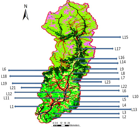
In order to get a true representative data of the entire study area, stratified random sampling was used after preliminary the reconnaissance in the entire study area. A map of the randomly selected sites were developed using ArcGIS 10 ArcMap utility (Figure 1) and different strata were identified using different physiographic features like water bodies, barren lands, alpine and glacial regions and built-up areas were masked-out in the map, to exclude them from the sampling. The Quadrats of 100 x 100 m were used for the
tree count and small 5 x 5 metre quadrats for the herbaceous sub-flora, as variation in the sampling size is allowed (Kent and Coker, 1996). All tree species of the minimum of three meter height were counted for all the plots (quadrats), geographical coordinates (GPS data) was recorded along with other metadata, i.e. Aspect, elevation and slope etc. using DX-GPS system of Red Hen technology.
Analysis of the Data
Fourteen different biodiversity indices were calculated using MS Excel and Biodiversity calculator (a small HTML coding package). The formulae used for the calculation of the indices are given in the Appendix 4. For in-depth analysis, interaction between variables such as average population size, presence of total organisms at the locations and the indices calculated, a multiple regression model was used for analysis using SPSS ver. 18 PASW (SPSS, 1997).
The following indices (Table 2) were used for further analysis to determine comparative vegetation structure between different locations. For each index, calculations have been carried out at the location level, not at the quadrat level as it would have been too much data to be handled. All locations were ranked on the bases of different Indices, and its relationship with the number of organisms of the location and species of the area was evaluated by the Linear multiple regression model.
Table 2: Ranks of all the locations based on the different indices (locations were coded as L1, L2, L3 to L23; for full name see Table 3)
|
Phyto-indices Ranking |
||||||||
|
Locations |
Total # Organisms |
Avg population size |
Simpson Index |
Dominance Index (D = 1 - Simpson) |
Shannon-Wiener Index (log) |
Menhinick’s Index |
Buzas and Gibson's Index |
Equitability Index |
|
L1 |
19 |
23 |
3 |
21 |
2 |
1 |
9 |
3 |
|
L2 |
12 |
17 |
21 |
3 |
16 |
4 |
18 |
18 |
|
L3 |
14 |
16 |
9 |
15 |
12 |
8 |
14 |
14 |
|
L4 |
20 |
20 |
4 |
20 |
10 |
10 |
2 |
2 |
|
L5 |
18 |
15 |
12 |
12 |
17 |
13 |
10 |
13 |
|
L6 |
22 |
21 |
8 |
16 |
11 |
6 |
5 |
5 |
|
L7 |
15 |
14 |
1 |
23 |
3 |
11 |
4 |
1 |
|
L8 |
7 |
12 |
2 |
22 |
1 |
7 |
11 |
8 |
|
L9 |
3 |
4 |
6 |
18 |
4 |
12 |
15 |
10 |
|
L10 |
23 |
22 |
13 |
10 |
15 |
9 |
6 |
9 |
|
L11 |
5 |
5 |
17 |
7 |
18 |
15 |
19 |
20 |
|
L12 |
1 |
1 |
20 |
4 |
21 |
21 |
22 |
22 |
|
L13 |
4 |
2 |
18 |
6 |
19 |
20 |
20 |
21 |
|
L14 |
17 |
6 |
19 |
5 |
20 |
22 |
1 |
7 |
|
L15 |
21 |
7 |
22 |
2 |
22 |
23 |
3 |
16 |
|
L16 |
2 |
3 |
14 |
11 |
14 |
14 |
21 |
19 |
|
L17 |
9 |
11 |
5 |
19 |
5 |
16 |
8 |
4 |
|
L18 |
10 |
9 |
7 |
17 |
8 |
18 |
7 |
6 |
|
L19 |
16 |
19 |
10 |
14 |
9 |
3 |
12 |
12 |
|
L20 |
8 |
10 |
15 |
9 |
13 |
17 |
16 |
17 |
|
L21 |
11 |
8 |
23 |
1 |
23 |
19 |
23 |
23 |
|
L22 |
6 |
13 |
16 |
8 |
7 |
5 |
17 |
15 |
|
L23 |
13 |
18 |
11 |
13 |
6 |
2 |
13 |
11 |
We have applied 18 different biodiversity indices to the vegetation of the area, the details of each is as follows: Dominance Index, which ranges from 0 (all taxa are equally present) to 1 (one taxon dominates the community completely); Simpson Index, which is 1-dominance, measures ‘evenness (equitability)’ of a community, ranges from 0 to 1; Shannon index (entropy): a diversity index that takes into account the number of individuals as well as number of taxa and varies from 0 for communities with a single taxon to high values for communities with many taxa with few individuals; Buzas and Gibson’s evenness; Berger-Parker dominance Index: which is simply the number of individuals in the dominant taxon relative to n (total number of taxa); Menhinick’s richness Index–the ratio of the number of taxa to the square root of a sample size; Margalef’s Richness Index; Equitability Index, which is the Shannon Diversity divided by the logarithm of number of taxa and measures the evenness; Gini Coefficient: which is a measure of the inequality of a distribution, a value of 0 expressing total equality and a value of 1 maximal inequality; and the Hill’s Numbers, which is a family of diversity numbers, corresponding to the ‘effective species richness’, in which rare species are given progressively less weight than common species (Table 3 and 4).
After ranking the locations with the biodiversity scores, they were regrouped and ranked. Hierarchical cluster analysis was also carried out for both location-location interaction and species-species interaction using SPSS version 18 (PASW).
Results
The various locations and number of species were depicted in Figure 1 indicating that Locations 8, 9 and 12 have higher tree species richness and offered a wider area for vegetation sampling. This initial assessment changed when cluster analysis was performed and the vegetation indices were calculated and outlined.
Cluster Analysis for Locations
The cluster analysis for similarities between locations, using average chi-square values was carried out. A visual interpretation of the dendrogram of the cluster analysis indicates 13 distinct locations on the basis of distribution of the tree species and their interactions using average linkage between them in the SPSS clustering algorithm.
Table 3: Show the selected sampling locations and their codes in the Swat Valley
|
Location Code |
Place name |
Location Code |
Place name |
|
L1 |
Landakay, Kota, Aboha, Gwaratai, Barikot |
L13 |
Marghuzarranzarosar, Sher Atraf |
|
L2 |
Nawagai, Krakar, Krakar Road, Karakarboundry |
L14 |
Mankial, Sur KarnMankial, JabaMankial, KozJaba, Badi Baba |
|
L3 |
Shingardar, wayna, Ghalegay, Odigram, Qambar, Amankot, Dandonoqala, Pajingram, Balogram |
L15 |
Kalam, ChiratKalam, Matiltan, Mahodand |
|
L4 |
Aqba, Saidu Sharif |
L16 |
Miandam proper |
|
L5 |
Goligram, Mian baba, Kokrai |
L17 |
Beshigram |
|
L6 |
Islam Pur, KhadraIslampur |
L18 |
Sulatanr, Rodingar |
|
L7 |
FatehPur |
L19 |
Kabal and the surrounding |
|
L8 |
Spal Bandai, Marghazar Road, Gul bandai, Grave yard, Mairagai, Mayna, Amluktal, Tarkana |
L20 |
Lalkoh |
|
L9 |
Marghazar proper |
L21 |
Ningwalai, Sher palam, Asharay |
|
L10 |
JawzosarMarghuzar |
L22 |
Topsin, Malam Jaba |
|
L11 |
Shagai, ChailShagai, SeraiShagai, Baligram |
L23 |
Sangar, Jambil, Kokarai |
|
L12 |
DoupIslampur |
- |
- |
Table 4: Eighteen different biodiversity indices used for all the locations
|
No. |
Index |
No. |
Index |
|
1 |
Simpson Index (∑(ni(ni-1)/(N(N-1)))) |
10 |
Alternate Simpson Index (∑((n/N))2) |
|
2 |
Dominance Index (D = 1 - Simpson) |
11 |
Alternate Dominance Index (D = 1 - Simpson) |
|
3 |
Reciprocal Simpson Index (1 / D) |
12 |
Alternate Reciprocal Simpson Index (1 / D) |
|
4 |
Shannon-Wiener Index (log) |
13 |
Berger-Parker Dominance Index |
|
5 |
Shannon-Wiener Index (ln) |
14 |
Inverted Berger-Parker Dominance Index |
|
6 |
Shannon-Wiener Index (adjusted) |
15 |
Margalef’s Richness Index |
|
7 |
Menhinick’s Index |
16 |
Rényi Entropy/Hill Numbers (0,1,2,∞) |
|
8 |
Buzas and Gibson's Index |
17 |
Gini Coeffificient |
|
9 |
Equitability Index |
18 |
ln() of Hill Numbers (0,1,2,∞) |
For details on biodiversity indices, see Harper (1999) and Magurran (2004)
These locations were grouped together along with their dominant tree species (Table 5 and Figure 2) of which locations L7 and L8 were miles away from each other but due to similar species composition and interaction they were agglomerated under the same branch as shown in the dendrogram. Location 13 (L13) shows a very distinct vegetation composition and looked almost an outlier appearing in the dendrogram at the bottom end. A closer look of the cluster (L3) shows that Cedrus deodara is a dominant tree species, in a close association with Pinus wallichiana subordinate species throughout the studied plots (Figure 3).
Table 5: Coefficients table of linear regression model: Equitability as dependent variable
|
Coefficientsa |
||||
|
Model |
T |
Sig. |
Collinearity Statistics |
|
|
Tolerance |
VIF |
|||
|
(Constant) |
22.145 |
.000 |
||
|
Total Number of Organisms |
-0.384 |
.705 |
.217 |
4.617 |
|
Average population size |
-1.104 |
.283 |
.217 |
4.617 |
a: Dependent Variable; Equitability Index
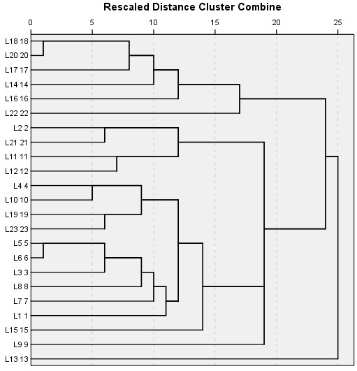
Figure 2: A hierarchical cluster analysis of the 23locations using average linkages method between groups. Rescaled distance measure was used as the linkage method for combining clusters
Cluster Analysis of Species Interaction
The results of the cluster analysis for the tree species at different locations indicate that some tree species grow in a very close association and will support a particular sub-flora (understory vegetation). Twelve distinct species-classes can be observed (Figure 3) of which two species, i.e. Eucalyptus spp. and Pinus roxburghii segregated in the dendrogram, suggesting that they would normally be found in close association forming an ecotone with other tree species. Pinus wallichiana, Picea smithiana and Abies pindrow can be grouped in one cluster, followed by Quercus incana and Cedrus deodara, neighbouring with Quercus dilatata. Acacia modesta show strong heterogeneity and did not share its habitat with any other constituent tree species at comparatively high elevation except with the lowland trees i.e. Morus spp. Melia azedarach and Ficus spp., respectively (Figure 3). Taxus baccata and Betula utilis are co-occurring species forming an association with Salix tetrasperma while, Quercus baloot and Aesculus indica are next associates, followed by Alnus nitida, Pyrus spp., Juglans and Salix babylonica at the lowland below the Acacia zone. A very close association can be observed between Ficus spp., Morus spp. and Melia azedarach, Platanus orientalis and Diospyrus lotus whereas; Olea ferruginea, Celtis caucasica and Cedrella serrata are branched together and show a similar trend in the arboreal forest.
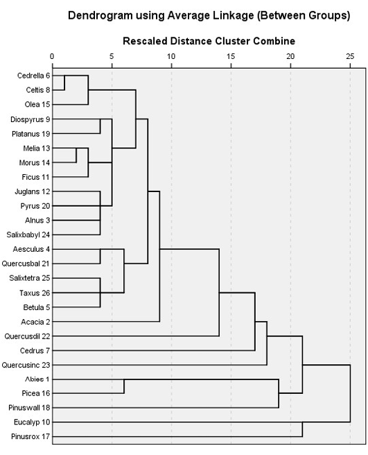
Figure 3: Twenty six different tree species were satisfactorily clustered into 12 groups using Chi-square between the sets of frequencies and species scores)
A ground-trothing analysis of the area also suggested the same pattern of tree association with the exception of Salix tetrasperma association with Taxus baccata and Betula utilis may be due to seeds or seedlings dispersal by floods in some northern regions of the Valley. It can also be observed that Pinus roxburghii and Eucalyptus spp. have the highest gain while the lowest gain was attained by Celtis caucasica respectively (Figure 3).The species are arranged in a close cluster according to their chances of appearance in the locations and their densities by the SPSS algorithm (Figure 4, 5 and 6).
Locations Ranking
For comparison of the diversity of different locations, heterogeneity in diversity, locations were ranked based on biodiversity measures (indices). Location 12 was ranked 1 in the categories of ‘total number of organisms’ and ‘population size’, but ranked 20th in the Simpson Index, 21st in the Shannon and Wiener and Menhinick’s Indices and 22nd in both Buzas and Gibson’s and Equitability Indices. In the Dominance Index it ranked 4th, indicates that these indices are not entirely dependent on the population size and species presence but also on the type of species and their relative abundance.
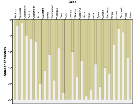
Figure 4: Cluster analysis (CA) of different tree species based on homogeneity/similarity of the species in the study area
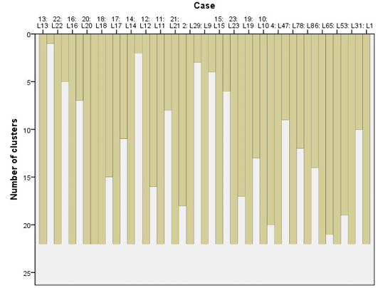
Figure 5: Cluster analysis of different locations based on similarity/homogeneity in the study areas
Location 7 was found to have the highest value (Rank = 1) for Simpson Index; Location 21 has the highest rank for Dominance Index, while Location 8 was having the top rank in Shannon-Wiener Index. Location 1 ranked 1st in the Menhinick’s Index and Location 14 has attained the highest ranking in Buzas and Gibson’s Index. The highest evenness was obtained by Location 7 in Equitability Index, which is in agreement with the Simpson Index. On the other hand Location 21 was found to have the lowest ranks in Simpsons, Shannon-Wiener, Buzas and Gibson’s, and Equitability indices (Table 2).
Linear Regression Model
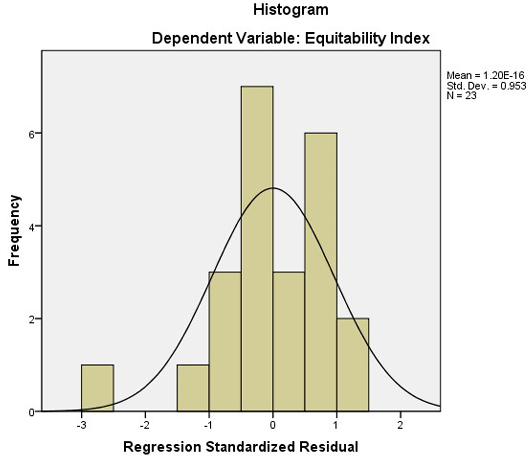
Figure 6: A histogram of regression model for Equitability index and average population size and number of organisms
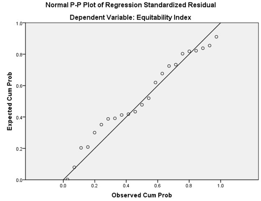
A linear regression model was fitted to the different indices to find out which indices are affected by the number of organisms in the plots and the average population of the area. The results of the regression analysis suggested that all the indices except Equitability Index is not affected by the combined effect of the number of species, and the average population size of the area (Table 5). The p-value is greater than the 0.5 significance level and thus the correlation is insignificant for both the number of organisms and average population size. The same pattern can also be observed in the PnP chart where the probability is deviating from the imagery straight line. The histogram for Equitability index shows a close match to a normal distribution, having the mean of 1.60, standard deviation of 0.953 for the sample size of 23 (see Figure 6 and 7).
Discussion and Conclusions
The Hindukush-Himalayan flora, especially, natural forests are under the influence of various kinds of disturbances, i.e. geological (landslides, soil erosion, earthquakes and anthropogenic (deforestation, grazing, lopping of tree branches for various uses, forest fires (Uniyal et al., 2010). The Swat District, part of the Himalaya-Hindukush series, is the biggest plant resources of the country, and is subjected to various types of the above biodiversity threats. It is a difficult place for biodiversity research, because of its rugged mountains and unique biodiversity. The severity of the disturbances may be due to the fact that the area is the remote part of the country and has a tribal social system in place, which overpowers the government grip on the area in some instances.
In order to preserve biodiversity, the first step would be to understand the biodiversity, the level, and consequences of the disturbance regimes, and the cost for the loss of biodiversity. In addition, we need to evaluate appropriate management strategies for the purpose of conservation. In this regard, biodiversity indices, (i.e. quantification of biodiversity), provide detail information about the intricate function of the ecosystem components. These indices can account for species being rare or common by evaluating the community health, and the change in the overall entropy of a community. In other words, the whole function of community can be quantified in numerical values and would be more elaborate than a simple description. The measure of biodiversity, strictly Functional Diversity (FD), is biologically of a great significance as it links species with their natural habitats, and their interaction with the rest of the population and community (Mason et al., 2005) thus, effecting the functionality of an ecosystem (Diaz et al., 2007). Biodiversity analysis is considerably important in areas where an altitude has stronger effect on the formation of microclimate and thus the change in the pattern of communities is more evident (Douglas and Bliss, 1977).
It is also a fact that woody plants alter the conditions for the ground flora by affecting the micro-environment and fertility of the soil (Weltzin and Coughenour, 1990). Trees and the ground flora are always in competition with each other for light, nutrients and water, but on the other hand trees provide important organic matter to the soil thus, increasing soil fertility (Belsky et al., 1989), which it turn increases the water-holding capacity of the soil, thus helping in the availability of water for the sub-flora (Dawson and Ehleringer, 1993). The effect of trees on the wind velocity, thermal balance and evapo-transpiration on the surface water is quite significant (Jose et al., 2008).
Species diversity and vegetation analysis studies can be very important for the understating of the intricate relationship between plants and their environment on a small spatial scale, as spatial heterogeneity may be caused by a small-scale environmental variation (Niemelä et al., 2006; Palmer and Dixon, 1990), or it may be due to the interaction between the species, as Pielou (1975) called “pattern diversity”. The question may be asked, as to what these interactions and relationships mean to us? According to Hill (1973), the interactions and diversity of an area can tell us about the stability, maturity, productivity, evolution, and spatial heterogeneity.
The graduated colour ranking shows that these different indices use different statistical approaches and have no real similarities. Comparison of the indices and using multi-indices for a community analysis is always helpful as biodiversity is a complex subject (Pielou, 1975) and the results are often useful if presented in graphs, tables and histograms (Usher, 1983).
There are some authors, for example, (Hurlbert, 1971) who are in absolute denial of biodiversity units and are against the use of biodiversity indices calculation, but others are in extreme favour of the term these measures and advocate on the use of these indices for the better understanding of ecological interaction (Hill, 1973).
It can be concluded from the results obtained here that biodiversity can change in different spatially different locations even in a short spatial range, and this finding is in agreement with (Niemelä et al., 2006). It was also concluded that the Equitability Index, which is the measure of evenness, is a good measure of understanding evenness and is independent of the combined effect of average population size and the number of organisms in the area. It can also suggest that, the individual Index can sometimes exaggerate the ground reality, thus the use of multiple indices and their comparison is advisable. The use of Simpson’s and Shannon Indices, along with the Equitability Index can give a reasonably clear picture of the biodiversity of the area, as some of the indices are widely used (Kent and Coker, 1996).
Some locations, like location 1, Location 4 and Location 7, which have high rankings in the indices (Table 4), should be further studied to identify the major reasons, while some poor diversified locations in many indices, like Location 21, should be given particular attention for promoting their biodiversity. It was also observed that the number of species in locations closer to the urban areas had more species, probably, due to the human interference in these communities by affecting the dominant species, as reported by Wohlgemuth et al. (2002). As such locations have their naturally occurring dominant species (Pinus wallichiana, Abies pindrow, Picea smithiana and Quercus spp.) cut down and replaced by exotic species like Eucalyptus lanceolatus and Eucalyptus globulus Labill., and other introduced species like Pinus roxburghii and in some cases Ailanthus altissima (Mill.) Swingle.
Finally, it was observed that every single pocket of vegetation in the District Swat shows varied degree of human interference and there is an urgent need for appropriate measures to be taken, to reduce the devastating trend. The solution could be the introduction of new trespassing laws, community mobilisation and education, along with the provision of basic needs of life to the local population.
Acknowledgments
We can confirm that all the authors have fully contributed in the development of the manuscript. They have worked simultaneously from data collection to analysis and interpretation. Although, at the data collection phase, Dr. Ali has contributed significantly, in the refinement and analysis phase, Dr. Nasrullah and Mr. Inayat contributions are highly significant. Miss Begum, Dr. Jury and Dr. Ahmad have contributed to the results interpretation and formatting of the manuscript. All authors have shared their expertise and knowledge in giving the final shape to the manuscript.
conflict of interests
We acknowledge the contribution of Mr. Shah Wazir Khan (a local Social worker and botany enthusiast) in helping with the field trips and establishment of socio- cultural interaction with the locals during the field trips.
authors’ contribution
We can confirm that this manuscrit ant its related research data has no conflict of interest. As there is no financial gain or loss to any individual or organization, directly or indirectly from the MANUSCRIPT.
References